Figures & data
Figure 1. Expansion muffler structure.
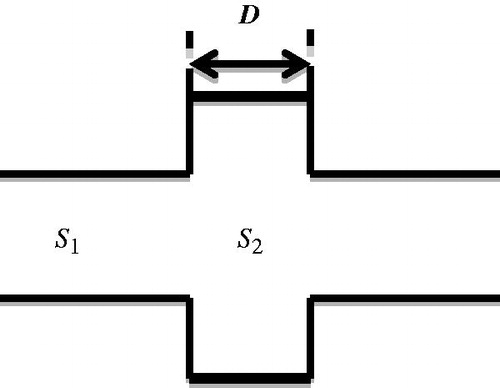
Figure 2. Side resonance structure.

Figure 3. Relationship between transmission coefficient and the length of the multi-section tube at 0.5 MHz (S12 = m × 1, with m = 1, 2, 3, 4, 5, and 5.4/2.4 indicated in blue, purple, red, green, grey, and black, respectively).
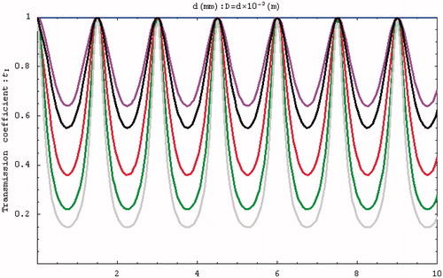
Figure 4. Relationship between transmission coefficient and frequency (S12 = m × 1, with m = 1, 2, 3, 4, 5, and 5.4/2.4 indicated in blue, purple, red, green, grey, and black, respectively).

Figure 5. Sound field distribution of a bilateral expansion tube for (a) , (b)
and (c)
(x in m, y in Pa).
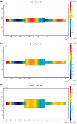
Figure 6. Sound field distribution of a bilateral contraction tube for .
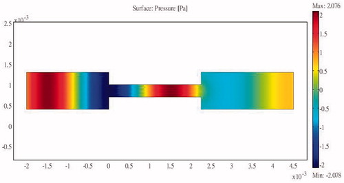
Figure 7. Sound field distribution of a unilateral expansion tube for (x in m, y in Pa).
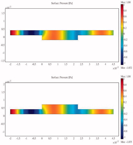
Figure 8. Sound field distribution of a unilateral contraction tube for (x in m, y in Pa).
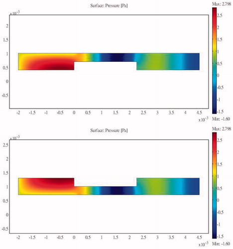
Figure 9. Basic concepts of the 2.25-cm sound-blocking structure.
Figure 10. Innovative sound-blocking structure for placement in front of the ribs.
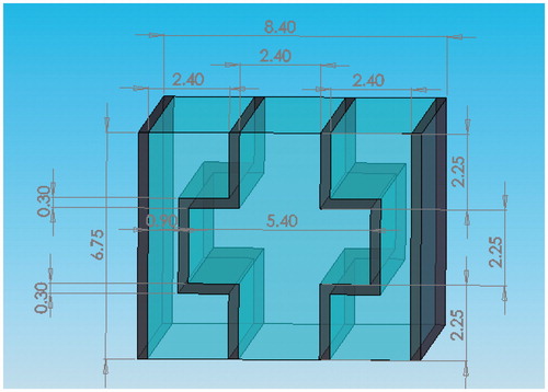
Figure 11. 3D views of the blocking structure frame.
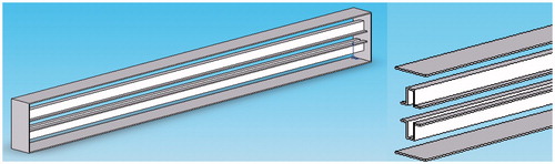
Figure 12. Dimensions of the resonator.
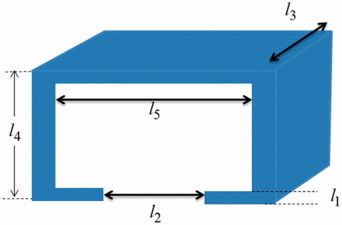
Figure 13. Sound intensity distribution for a unilateral side resonance structure in the upstream region of the tube.
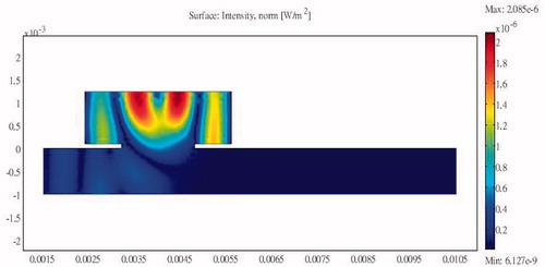
Figure 14. Sound intensity distribution for a unilateral side resonance structure in the downstream region of the tube.
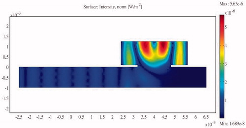
Figure 15. Minimising interference using a combination of side resonance structures.
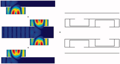
Figure 16. 3D diagrams of the combined side resonance structures.
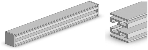
Figure 17. Overall schematic diagram of the structure and the sound propagation path.
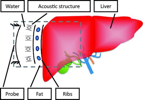
Table 1. Elasticity matrix (ordering: x, y, z, yz, xz, xy), in Pa.
Table 2. Coupling matrix, in C/m2.
Table 3. Relative permittivity.
Table 4. Media parameters along the sound propagation path.
Figure 18. Sound field simulation in the absence of protection.
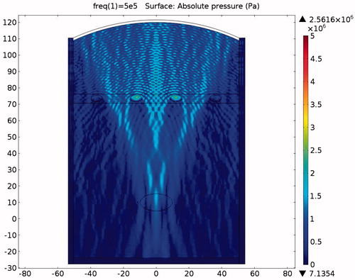
Figure 19. Sound intensity simulation in the absence of protection (x axis is in mm, y axis is in Pa).
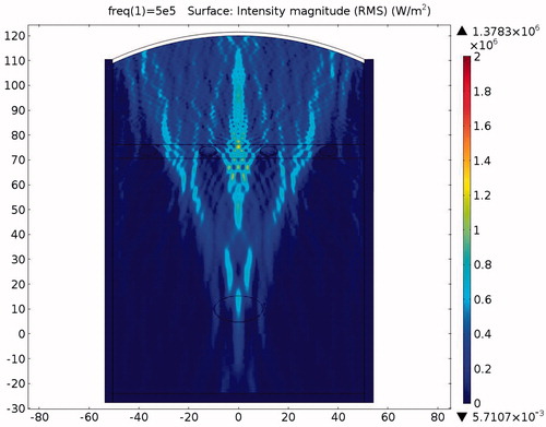
Figure 20. Temperature distribution in the absence of protection after a 0.1-s ablation (x axis is in mm, y axis is in Pa).
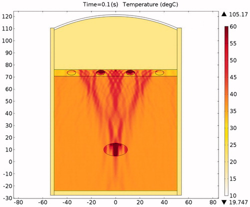
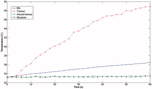
Figure 21. Temperatures of rib and tumour after 0.1-s ablation time.
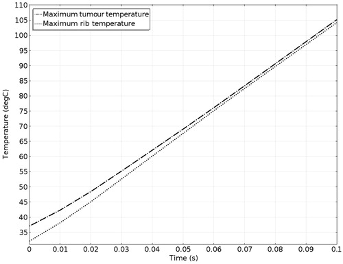
Figure 22. Sound field simulation in the presence of the expansion muffler structure (x axis is in mm, y axis is in Pa).
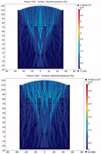
Figure 23. Sound intensity simulation in the presence of the expansion muffler structure (x axis is in mm, y axis is in Pa).
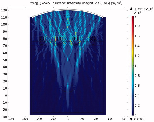
Table 5. Thermal characteristics of various materials.
Table 6. Arterial blood temperature and perfusion rate.
Figure 24. Ablation temperature distribution in the presence of the expansion muffler structure after a 0.1-s ablation (x axis is in mm, y axis is in Pa).
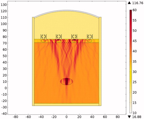
Figure 25. Temperatures of the ribs and the tumour after a 0.1-s ablation.
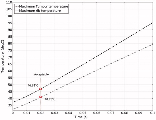
Table 7. Temperatures of rib and tumour after a 0.02-s ablation.
Figure 26. Sound field simulation in the presence of the resonator structure (x axis is in mm, y axis is in Pa).
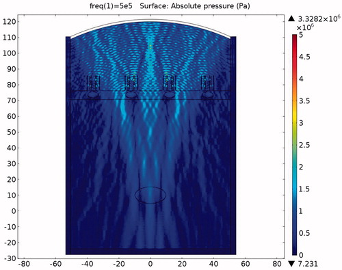
Figure 27. Close-up view of the pressure distribution around a single rib and resonator structure (x axis is in mm, y axis is in Pa).
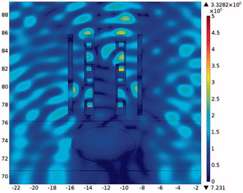
Figure 28. Sound intensity simulation in the presence of the resonator structure (x axis is in mm, y axis is in Pa).
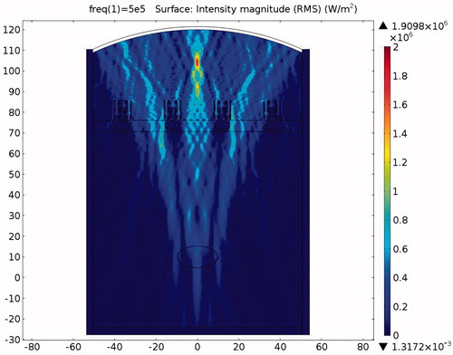
Figure 29. Temperature distribution in the presence of the resonator structure after a 0.1-s ablation (x axis is in mm, y axis is in Pa).
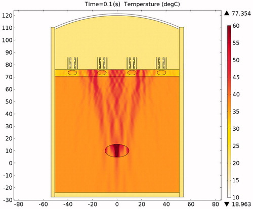
Figure 30. Temperatures of the rib and tumor after a 0.1-s ablation time.
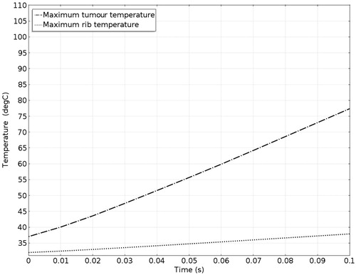
Figure 31. Experimental setup for HIFU rib sparing tests (DAQ: Data Acquisition, PC: Personal Computer).
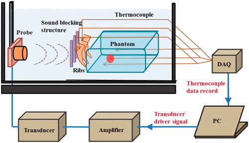
Figure 32. Ablation with the rib protective structure in place.
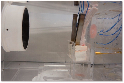
Figure 33. Ablation without protection.
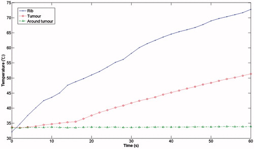
Figure 34. Ablation with the rib protective structure in place.