Design and characterisation of miniaturised cavity-backed patch antenna for microwave hyperthermia

Figures & data

Figure 1. A 3D numerical model of the probe-fed cavity-backed resonant patch antenna studied in EM simulation software, HFSS®.

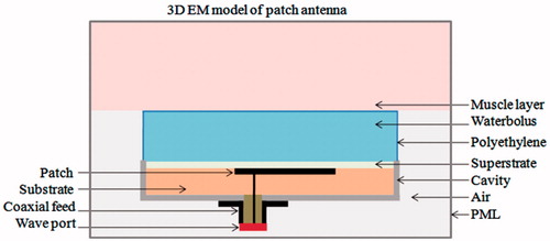
Table 1. Material properties of model domains^a.

Material domain	Relative permittivity	Conductivity (S/m)	Density, (kg/m^3)
DI water^b	78	0.805	1000
Air	1.006	0	1.1
Muscle^c	56	0.8	1000
Aluminium	1	38 × 10^6	2689
Copper	1	58 × 10^6	8933
Teflon	2.1	0.0005	2250
Polyethylene	2.25	0	930

^aH/m.

^bMeasurement at 434 MHz.

^c[16] value at 434 MHz.

Figure 2. Evolution of the compact probe-fed patch antenna inside a metal enclosure. (A) Rectangular patch, (B) folded C-type patch and, (C) C-type folded patch with shorting post near the feed.

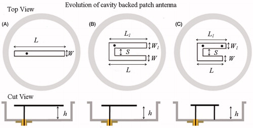
Table 2. Sweep range for the design parameters of cavity-backed rectangular patch (Figure 2A).

Physical dimensions	Range (mm)
Patch length (L)	26–32
Substrate height (h)	9–11
Superstrate height (h2)	2–5
Patch width (W)	2–4
Feed position from origin:
	xf	3–9
	yf	6.3
Bolus thickness (h1)	20–50

Figure 3. Experimental set up for antenna SAR measurement.

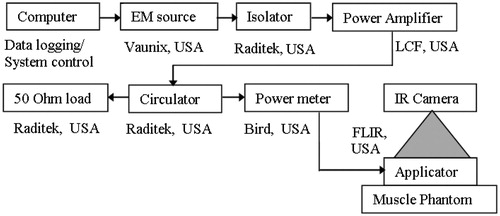
Figure 4. Influence of the design parameters of the cavity-backed rectangular patch namely, (A) patch length (L), (B) height (h.) and (C) width (W) on return loss . (D) Return loss of the optimised cavity-backed patch with S₁₁ = −17.31 dB at 434 MHz satisfying the design criteria (L = 28.5 mm, h = 10 mm, W = 3 mm).

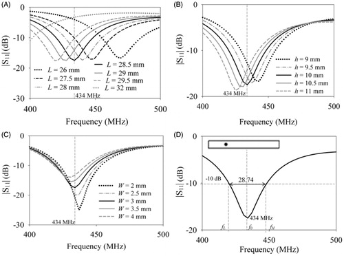
Figure 5. Simulation results of the cavity-backed folded C-type patch of Figure 2(B). Influence of the folded patch lengths namely, (A) the first (L) and (B) second arms (L₁) on antenna return loss ; (C) return loss for the optimised C-type patch (L = 26 mm, L₁ = 26 mm, h = 10 mm, W = 3 mm, S = 3 mm), and (D) normalised electric field at 434 MHz in the antenna near field.

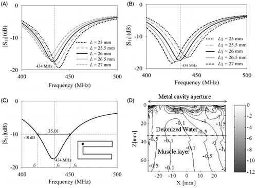
Figure 6. Simulation results of the miniaturised patch with metal enclosure, folded C-type arm and shorting post near the feed. Influence of the lengths of the (A) first (L) and(B) second arms (L₁) on antenna return loss ; (C) influence of the spacing between shorting post and feed Δx = 16 mm and (D) return loss of the optimised patch (L = 20 mm, L₁ = 22 mm, h = 10 mm, W = 3 mm, S = 3 mm).

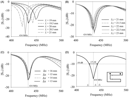
Figure 7. Orientation of induced current density on the patch surface for the optimised (A) cavity-backed rectangular patch, (B) C-type cavity-backed patch without shorting post, (C) with shorting post; (D) orientation of electric field vector radiated by the miniaturised cavity-backed folded C-type patch with shorting post in the antenna near-field.

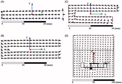
Figure 8. Prototypes of the miniaturised antenna for microwave hyperthermia. (A) C-type folded patch with a shorting post near the feed inside a metal cavity; (B) prototype 1 with flexible 0.3 mm thick PVC water bolus; (C) prototype 2 with rigid side wall to maintain constant bolus thickness and a flexible PVC film at the skin-contacting side.

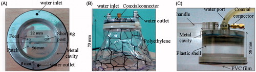
Figure 9. Comparison between return loss measurements of the fabricated miniaturised patch and simulation. Return loss measurements of (A) prototype 1 with flexible water bolus for polyacrylamide phantom, and (B) prototype 2 with fixed water bolus height (h₁) and plastic outer shell for no load, poly acrylamide and gelatin phantoms.

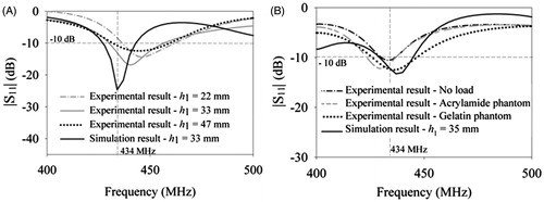
Figure 10. Normalised SAR along the depth of muscle phantoms (XZ plane) for varying pulse duration, Δt. SAR measurements of polyacrylamide gel phantom for (A) 45 s, (B) 60 s and (C) 90 s, (D) simulation results for muscle tissue, (E) normalised SAR of gelatin phantom for Δt = 60 s, (F) comparison of measured and simulated SAR depth profiles.

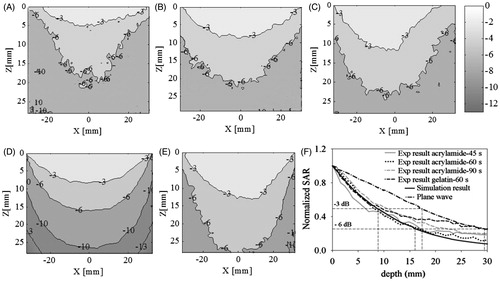
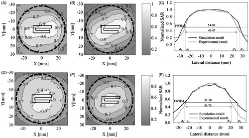
Figure 11. Normalised SAR at a given depth in muscle phantoms (XY plane). SAR at 5 mm depth for (A) polyacrylamide gel phantom, Δt = 60 s and, (B) simulation result; (C) comparison between measured and simulated SAR profiles along y = 0 mm. SAR surface distribution at 20 mm depth for (D) gelatin phantom, Δt = 60 s, (E) simulation result for muscle tissue, (F) comparison between measured and simulated SAR profiles along y = 0 mm. The dotted black line indicates the outer circumference of the metal cavity (56 mm diameter with 8 mm wall thickness).

Table 3. Summary of maximum rise in temperature, ΔT_max, maximum SAR (SAR_MAX, (°C)) and normalised SAR for polyacrylamide gel and gelatin phantoms for varying heating durations and comparison with simulation results.

				SAR coverage (cm^2)
Phantom	Duration Δt (s)	ΔTmax, (°C)	SARmax (W/kg)	−3 dB	−6 dB
SAR plane XZ (depth) y = 0 mm
Polyacrylamide C = 3475 J/g°C, ρ = 1233 kg/m^3	45	1.92	220.19	1.95	7.15
	60	2.33	199.98	3.21	9.07
	90	3.29	189.15	4.02	11.42
Simulation			298.00	3.09	6.42
Gelatin C = 4187 J/g°C, ρ = 1000 kg/m^3	60	5.10	355.89	5.62	13.70
Simulation			367.00	3.95	7.97
SAR plane XY (surface) z = 5 mm
Polyacrylamide	60	1.00	114.68	23.12	43.75
Simulation			200.00	18.58	27.87
SAR plane XY (surface) z = 20 mm
Gelatin	60	0.96	66.99	25.22	37.28
Simulation			65.60	18.00	36.00

Gabriel S, Lau RW, Gabriel C. The dielectric properties of biological tissues: III. Parametric models for the dielectric spectrum of tissues. Phys Med Biol 1996;41:2271–93

 PubMed Web of Science ®Google Scholar