Hyperthermia treatment planning for cervical cancer patients based on electrical conductivity tissue properties acquired in vivo with EPT at 3 T MRI

Figures & data

Table 1. Thermal properties assigned to different tissue types used for hyperthermia treatment planning. Values are based on [42,43].

Tissue type	Density ρ (kg m^−3)	Perfusion Wb (kg m^−3 s^−1)	Thermal conductivity k (W m^−1 K^−1)	Specific heat capacity c (J kg^−1 K^−1)
Air	1.29	0	0.024	10 000*
Bone	1595	0.12	0.65	1420
Muscle	1050	3.6	0.56	3639
Fat	888	1.1	0.22	2387
Cervical tumour	1050	1.8	0.56	3639
Bladder	1050	3.6	0.56	3639

*The value of c used for air was ten times too high in order to allow larger time steps in thermal computations. This has a negligible effect on the steady-state temperature (< 2 × 10⁻⁵ °C).

Table 2. Electrical properties assigned to different tissue types at 70 MHz used for hyperthermia treatment planning. Values are based on Gabriel et al. [5,42,43,48]. Bold type denotes electrical conductivity values based on EPT [32].

	Electrical conductivity σ (S/m)
Case	I	II	III	IV	V	VI	Relative permittivity ɛr
Tissue type
Air	0	0	0	0	0	0	1
Bone	0.05	0.05	0.05	0.05	0.05	0.05	10
Muscle	0.75	0.93 (± 0.14)	0.93	0.75	0.93	0.75	75
Fat	0.06	0.06	0.06	0.06	0.06	0.06	10
Cervical tumour	0.75	1.00 (± 0.15)	1.00	0.75	0.75	1.00	65
Bladder	0.93	1.80 (± 0.54)	2.50	1.80	0.93	0.93	77

Table 3. An overview of the dielectric data sets used for optimisation (second row) and the dielectric data set on which the optimised antenna setting was applied (third row). Data sets are listed in Table 2. Results are depicted in Figures 1–4.

Label	I→I	I→II	I→III	I→IV	I→V	I→VI	I → IIɛr, m = 60 − 90	II→II
Optimisation dataset	I	I	I	I	I	I	I	II
Actual parameters	I	II	III	IV	V	VI	IIɛr, m = 60 − 90	II
Figure	1,2,3,4	1,2	1,2	1,2	1,2	1,2	3	4

Figure 1. Tumour T90 (top) and T50 (bottom) in patients 1–5 for AMC-4 and AMC-8 system. The white bar represents the optimised case for properties based on literature values. Using the same antenna settings, the tumour temperature for different cases are computed and represented by other bars.

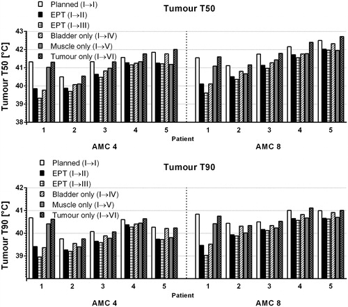
Figure 2. Tumour SAR in patients 1–5 for AMC-4 and AMC-8 system. The white bar represents the optimised case for properties based on literature values. Using the same antenna settings, the tumour temperatures for different cases are computed and represented by other bars.

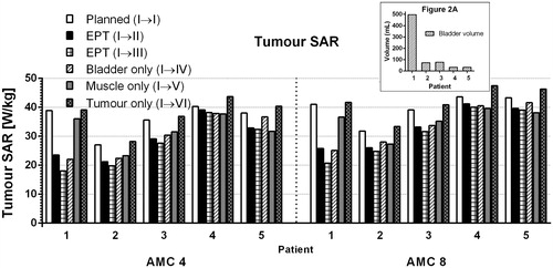
Figure 3. Tumour T90 in patients 1–5 for AMC-4 and AMC-8 system. The white bar represents the optimised case for properties based on literature values. The error bars represent the minimum and maximum tumour T90s when using highest and lowest conductivity values, respectively, as presented in case II (Table 2).

Figure 4. Tumour T90 for patients 1 (top) and 5 (bottom) for optimised cases with literature value (white) and for EPT-based conductivity values of muscle, cervical tumour and bladder filling (black). The other bars represent tumour T90 values for different values of muscle permittivity.

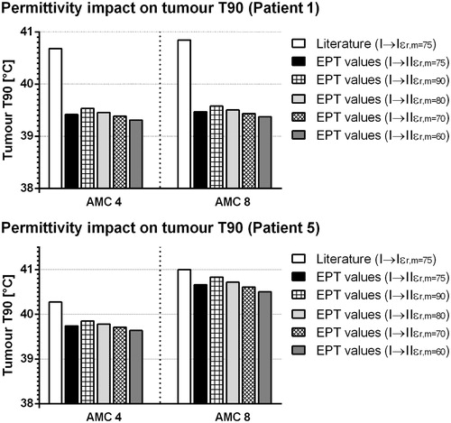
Figure 5. Tumour T90 for patients 1–5 based on literature values (white) and on EPT-based conductivity values (grey). The applied antenna settings were computed separately by temperature-based optimisation for both cases.

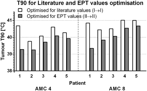
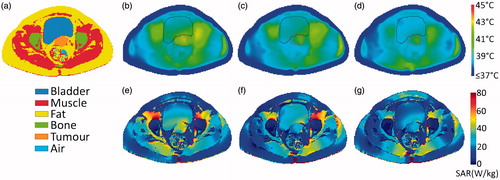
Figure 6. An example of the resulting temperature distribution of patient 1 corresponding to transverse slice (a) for the case, (b) planned with literature values (I→I), and (c) the case where the same antenna settings are applied on the EPT-based model (I→II). In (d) is shown the distribution resulting for temperature-based optimisation based on EPT model (II→II). (e–g) The corresponding SAR distributions are shown.

Hasgall P, Di Gennaro F, Baumgartner C, Neufeld E, Gosselin M, Payne D, et al. IT’IS database for thermal and electromagnetic parameters of biological tissues, Version 2.6, January 13th, 2015. Available at www.itis.ethz.ch/database

 Google Scholar

ESHO Taskgroup Committee 1992 Treatment planning and modelling in hyperthermia Task Group Report of the European Society for Hyperthermic Oncology. Rome (Italy): Tor Vergata; 1992.

 Google Scholar

Gabriel C. Compilation of the dielectric properties of body tissues at rf and microwave frequencies. Brooks Air Force Tech Rep 1996;AL/OE-TR:0037.

 Google Scholar

Andreuccetti D, Fossi R, Petrucci C. An Internet resource for the calculation of the dielectric properties of body tissues in the frequency range 10 Hz–100 GHz. Florence (Italy): IFAC-CNR; 1997. Available at http://niremf.ifac.cnr.it/tissprop/.

 Google Scholar

Balidemaj E., de Boer P., van Lier ALHMW., Remis RF., Stalpers LJA., Westerveld GH., Nederveen AJ, van den Berg CAT and Crezee J In vivo electric conductivity of cervical cancer patients based on maps at 3T MRI. Physics in Medicine and Biology 2016;61:1596-1607.

 PubMed Web of Science ®Google Scholar