Dynamic MLC tracking of moving targets with a single kV imager for 3D conformal and IMRT treatments

Figures & data

Figure 1. Schematic showing the gantry angles for the five fields (F1-F5), the 120° pre-treatment gantry rotation, and the 72° inter-field gantry rotations. Fluoroscopic kV images were acquired during the entire procedure and used for DMLC tracking of the moving phantom.

Figure 2. Example of data from a typical tracking experiment for a lung tumor trajectory. From top to bottom the curves show the following as function of time: gantry angle, beam-on status, and requested MLC aperture center position perpendicular and parallel to the MLC leaf motion direction. All data were extracted from Dynalog files recorded during the experiment.

Figure 3. Example of tracking experiment for lung tumor trajectory. (a, b) Phantom motion (black) and real-time estimated trajectory at the time of imaging (blue) and at the time of beam correction (i.e. after 570 ms prediction) (red). The data are shown in room coordinates (a) and in beam's eye view of the treatment beam (b). In (b), the real-time estimations are only shown for beam-on periods. (c) Position of marker (black) and beam aperture center (red) perpendicular and parallel to the MLC leaves as determined from portal images. (d) Gantry angle. The numbers specify the rms position estimation error before/after prediction (a, b) and the rms tracking error (c).

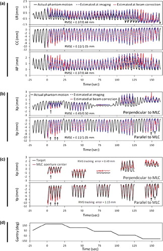
Figure 4. Example of tracking experiment for prostate trajectory. (a) Phantom motion (black) and real-time estimated trajectory (blue) in room coordinates. (b) Phantom motion (black) and real-time estimated trajectory at the time of imaging (blue) and 570 ms later (red) in beam's eye view of the treatment beam. (c) Position of marker (black) and beam aperture center (red) perpendicular and parallel to the MLC leaves as determined from portal images. (d) Gantry angle. The numbers specify the rms position estimation error at imaging (a) or at imaging/570 ms after imaging (b), and the rms tracking error (c).

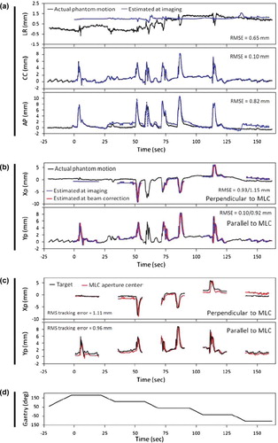
Table I. Results of experiments [and simulations hereof shown in brackets]. Rms of position estimation errors, tracking errors and target displacement.

	Real-time position estimation error at time of …							Tracking error in MV images		Target motion
	Imaging					Imaging + 570 ms
	LR	CC	AP	Xp	Yp	Xp	Yp	Xp	Yp	Xp	Yp
12 experiments with thoracic/abdominal tumor trajectories:
Mean RMSE:	0.47	0.10	0.39	0.57 [0.42]	0.10 [0.001]	0.89 [0.76]	1.00 [0.99]	0.85	1.09	1.3	1.8
Max RMSE:	0.92	0.21	0.73	1.08 [1.12]	0.21 [0.002]	2.3 [2.2]	2.1 [2.3]	2.1	2.4	4.2	4.5
5 experiments with prostate trajectories:
Mean RMSE:	0.29	0.09	0.53	0.55 [0.45]	0.09 [0.002]	0.62 [0.54]	0.37 [0.35]	0.59	0.49	1.6	1.8
Max RMSE:	0.65	0.13	0.82	0.93 [0.94]	0.13 [0.006]	1.15 [1.16]	0.92 [0.89]	1.11	0.97	2.6	4.2

Mean and maximum root-mean-square error (RMSE) in the target position estimation at the time of imaging and at the time of beam correction. RMS of the tracking error in portal images and of the target displacement. All units are mm. Xp and Yp are the projected position in MV beam's eye view perpendicular and parallel to the MLC leaf direction, respectively.

Figure 5. Root-mean-square errors in 12 experiments for thorax/abdomen tumor trajectories versus the rms errors in simulations of the same experiments.

Figure 6. Root-mean-square errors in five experiments for prostate trajectories versus the rms errors in simulations of the same experiments.

Table II. Simulation results. Rms of position estimation errors and target displacement.

	Real-time position estimation error at time of …
	Imaging					Imaging+285 ms		Imaging+570 ms		Target motion
	LR	CC	AP	Xp	Yp	Xp	Yp	Xp	Yp	Xp	Yp
160 thoracic/abdominal tumor trajectories:
Mean RMSE (20s per field):	0.20	0.001	0.21	0.30	0.001	0.44	0.59	0.55	0.90	0.80	1.64
Max RMSE (20s per field):	1.30	0.01	0.78	1.30	0.02	1.9	3.9	2.4	5.8	4.2	8.0
Mean RMSE (60s per field):	0.23	0.001	0.25	0.35	0.001	0.46	0.59	0.56	0.90	0.83	1.69
Max RMSE (60s per field):	1.06	0.01	1.01	1.33	0.009	1.9	2.8	2.4	4.1	3.6	7.5
548 prostate trajectories:
Mean RMSE (20s per field):	0.16	0.001	0.23	0.28	0.001	0.29	0.11	0.30	0.16	0.62	0.67
Max RMSE (20s per field):	1.09	0.004	1.17	1.41	0.008	1.42	0.63	1.43	0.91	5.7	5.5
Mean RMSE (60s per field):	0.22	0.001	0.31	0.38	0.001	0.40	0.12	0.40	0.17	0.86	0.92
Max RMSE (60s per field):	2.5	0.01	3.3	4.1	0.01	4.1	0.37	4.1	0.56	4.4	5.4

Mean and maximum of the rms target position estimation error at the time of imaging and at the time of beam correction in case of 285 ms and 570 ms tracking system latencies. All units are mm. Xp and Yp are the projected position in MV beam's eye view perpendicular and parallel to the MLC leaf direction, respectively.