Evaluation of image quality for different kV cone-beam CT acquisition and reconstruction methods in the head and neck region

Figures & data

Table I. Detailed CBCT image acquisition parameters.

Acquisition mode	Abbreviation	Peak voltage (kVp)	Tube current (mA)	Exposure time (ms)	Rotation range (deg)	Number of projections*	Exposure (mAs)*
Standard-dose head	SDH	100	20	20	200	372	149
Standard-dose head full scan	SDHFS	100	20	20	360	669	268
High-quality head	HQH	100	80	25	200	372	744
High-quality head full scan	HQHFS	100	80	25	360	669	1338
OBI1.3 full scan	OBI13FS	125	80	25	360	669	1338

*Average number for clockwise and counter clockwise CBCT scan direction.

Figure 1. Representative slices of Catphan 504 phantom used to assess (a) HU uniformity, (b) HU verification and linearity, contrast, and (c) high contrast spatial resolution.

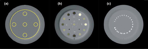
Figure 2. Plot of the nominal HU values of the seven Catphan inserts as a function of translated raw image values after FFE reconstruction for the five CBCT modes. Before the plotting, the raw image values were translated by adding a constant of 890 and 900 for 100 kV and 125 kV modes, respectively. Solid lines stem from linear regression fits shown in the figure legends.

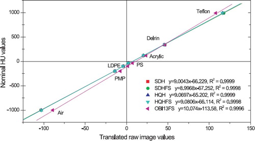
Figure 3. Mean HU value and standard deviation from the distribution of values within the central slice of the uniform disk in Catphan for five CBCT modes and two CT scanners. CBCT scans underwent two different reconstructions and CT scans were performed with two different exposures.

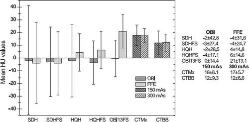
Figure 4. (a) Integral nonuniformity (IN) and (b) uniformity index (UI) of five CBCT modes and two CT scanners. CBCT scans underwent two different reconstructions and CT scans were performed with two different exposures. Error bars correspond to +/− one standard deviation for mean values over five axial slices.

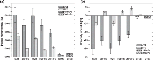
Figure 5. Difference between measured and nominal HU values in the seven inserts in Catphan 504 for five CBCT modes reconstructed with OBI and FFE. Error bars correspond to +/− one standard deviation for mean values over five axial slices.

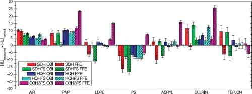
Figure 6. Contrast-to-noise ratio (CNR) of the seven Catphan 504 inserts for five CBCT modes reconstructed with OBI and FFE, and two CT scanners with two different exposures. Error bars correspond to +/− one standard deviation for mean values over five axial slices.

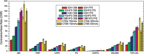
Figure 7. Low contrast visibility from Equation 4 for five CBCT modes reconstructed with OBI and FFE, and two CT scanners with two different exposures. Error bars correspond to +/- one standard deviation for mean values over five axial slices.

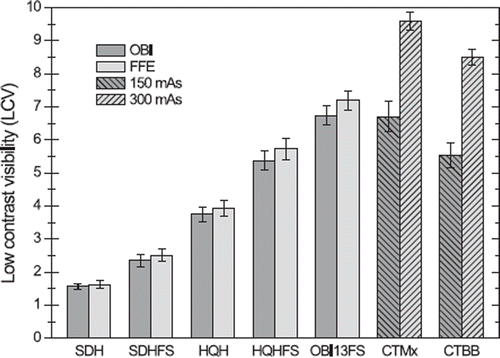
Table II. MTF for five CBCT modes reconstructed with OBI and FFE, and two CT scanners with two different exposures. MTF values at 50% (f₅₀) and 10% (f₁₀) are shown in line pairs/cm.

	SDH		SDHFS		HQH		HQHFS		OBI13FS		CTMx		CTBB
MFT	OBI	FFE	OBI	FFE	OBI	FFE	OBI	FFE	OBI	FFE	150 mAs	300 mAs	150 mAs	300 mAs
f50 lp/cm	5.42	5.48	4.95	4.98	5.39	5.46	4.61	4.66	4.47	4.49	3.44	3.39	3.69	3.67
f10 lp/cm	9.39	9.34	8.56	8.54	9.27	9.26	8.02	8.02	7.72	7.71	6.10	5.99	6.68	6.66

Figure 8. Reconstructed anthropomorphic head phantom images from (a) CT, (b)–(f) CBCT OBI, and (g)–(k) CBCT FFE (level =100 HU, window = 600 HU). From left to right the CBCT stem from SDH, SDHFS, HQH, HQHFS and OBI13FS reconstructions, respectively.

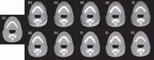
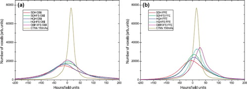
Figure 9. The distribution of HU values from −200 HU to 200 HU in CBCT of anthropomorphic head phantom for (a) OBI and (b) FFE reconstruction. CT data have been added on both for comparison.