Figures & data
Table I. Parameter values used in the USC model.
Figure 1. Typical inhomogeneous dose distribution within the PTV as used in SBRT. Numbers in the OARs refer to the different cases described in the three sections of the Material and methods.
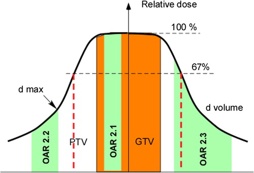
Figure 2. a. Dose volume histograms for ipsilateral lung-GTV with a low (A), medium (B), and high (C) mean lung dose. To better distinguish the lines at small relative lung volumes, they are shown in logarithmic scale, with an insert in linear scale. b. Dose distributions for three patients with a low (A), medium (B), and high (C) mean lung dose. Blue isodose is the prescription isodose (15 Gy at 65%) at the periphery of the PTV, green is 50%, yellow 32%, and grey 16%. Red isodoses are 80%, 87%, and 93% of 22 Gy. PTV and GTV are shown by red and orange lines.
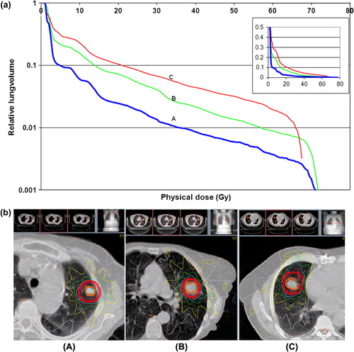
Figure 3. Isoeffect curves calculated for tumour and normal tissue using LQ (dotted lines) and USC (full lines) for fractionation correction. In figure a) with dose/fraction and in figure b) with number of fractions as independent variable.
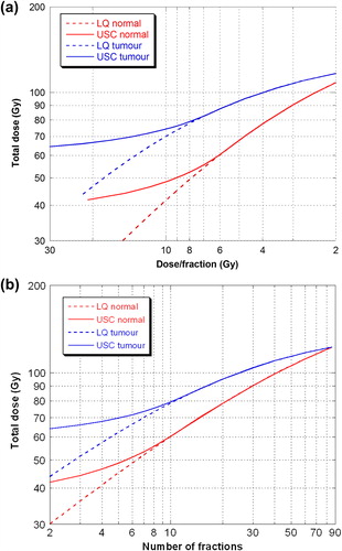
Figure 4. a. Cell survival calculated for normal tissue, for constant cell survival in the tumour. The left panel gives the results in absolute numbers, and the right panel gives the cell survival relative to that at 3 fractions, at which the prescribed central dose is 22 Gy. The different lines give the result for different maximum doses to the OAR relative to the dose to GTV. The USC model is shown by full lines and the LQ model with dotted lines. b. Gain in tolerance dose to OAR, with numbers of fractions relative to that for 3 fractions. The different lines give the results for different maximal doses to the OAR relative to the prescribed central dose. The USC model is represented by full lines and LQ model with dotted lines.
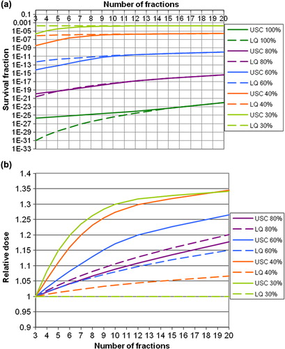
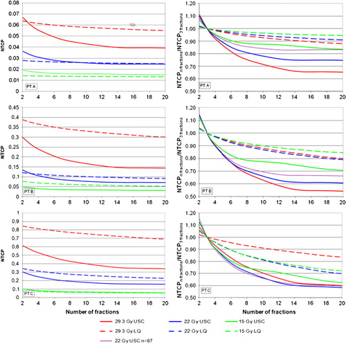
Figure 5. NTCP versus number of fractions, for RP2+ for a constant cell survival in the tumour for three different prescribed central tumour doses (3 × 29.3 Gy, 3 × 22 Gy and 3 × 15 Gy). Three patients are used in the calculations: one with a low (PT A), one with a medium (PT B), and one with a high (PT C) mean lung dose. The USC model is shown by full lines and the LQ model by dotted lines. Note the different scales on y-axes for NTCP.