A method for differentiating cancer prevalence according to health status, exemplified using a population-based sample of Italian colorectal cancer cases

Figures & data

Figure 1. Lexis diagrams illustrating the methods used to combine data from the cohort and period approaches to produce a fictitious cohort on which differentiated prevalence was estimated. (a) Illustration of cohort (ABCD) and period (EDWV) approaches; (b) Construction of fictitious cohort (ABXY) combining data from the cohort and period approaches; (c) Estimation of differentiated prevalence from fictitious cohort.

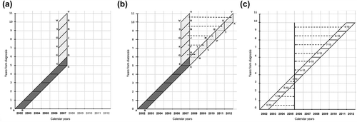
Table I. Health status distribution of colon and rectal cancer cases collected for the period approach. All ages and both sexes.

Interval	Colon cancer									Rectal cancer
	Prevalent cases analyzed	Deaths due to colorectal cancer		Deaths due to other causes*		Cases considered ill at least one day of period		Cases with no evidence of disease for all days in period		Prevalent cases analyzed	Deaths due to colorectal cancer		Deaths due to other causes*		Cases considered ill for one day at least of period		Cases with no evidence of disease for all days in period
(5,7)	30	0	–	1	3%	4	13%	25	84%	30	1	3%	1	3%	1	3%	27	91%
(6,8)	29	0	–	0	–	2	7%	27	93%	31	3	10%	0	–	2	6%	26	84%
(7,9)	31	0	–	1	3%	0	–	30	97%	29	0	–	1	4%	3	10%	25	86%
(8,10)	29	0	–	1	4%	1	4%	27	92%	32	0	–	0	–	2	6%	30	94%
(9,11)	30	0	–	1	3%	0	–	29	97%	27	0	–	0	–	3	11%	24	89%

*Including cases with cause of death unknown.

Table IIa. Colon cancer: Health status distribution of fictitious cohort by each annual intervals. All ages, both sexes.

Approach	Interval (j,j + 1)	Nj	D^cj,j + 1		D^ocj,j + 1		Ij,j + 1		Hj,j + 1
		Patients alive at beginning of interval	Deaths due to colorectal cancer		Deaths due to other causes*		Cases considered ill at least one day in interval		Cases with no evidence of disease for entire interval
Cohort	(0,1)	300	66	22%	7	2%	227	76%	0	–
	(1,2)	227	23	10%	2	1%	35	15%	167	74%
	(2,3)	202	16	8%	2	1%	26	13%	158	78%
	(3,4)	184	8	4%	4	2%	18	10%	154	84%
	(4,5)	172	14	8%	5	3%	16	9%	137	80%
Period	(5,6)	153	4	3%	0	–	20	13%	129	84%
	(6,7)	149	0	–	5	3%	10	7%	134	90%
	(7,8)	144	0	–	5	3%	0	–	139	97%
	(8,9)	139	0	–	0	–	5	4%	134	96%
	(9,10)	139	0	–	9	7%	0	–	130	93%

D^c_{j,j + 1}: patients alive in j who died of studied cancer before j + 1.

D^oc_{j,j + 1}: patients alive in j who died of other causes before j + 1.

I_{j,j + 1}: patients alive in j ill on at least one day before j + 1.

H_{j,j + 1}: patients alive in j without evidence of cancer before j.

*Including cases with cause of death unknown.

Table IIb. Rectal cancer: Health status distribution of fictitious cohort by each annual intervals. All ages, both sexes.

		Nj	D^cj,j + 1		D^ocj,j + 1		Ij,j + 1		Hj,j + 1
Approach	Interval (j,j + 1)	Patients alive at beginning of interval	Deaths due to colorectal cancer		Deaths due to other causes*		Cases ill at least one day in interval		Cases with no evidence of disease for entire interval
Cohort	(0,1)	301	77	25%	2	1%	222	74%	0	–
	(1,2)	222	27	12%	0	–	60	27%	135	61%
	(2,3)	195	26	13%	3	2%	23	12%	143	73%
	(3,4)	166	12	7%	1	1%	26	16%	127	76%
	(4,5)	153	3	2%	4	3%	23	15%	124	80%
Period	(5,6)	147	6	4%	8	5%	5	4%	128	87%
	(6,7)	133	4	3%	0	–	5	4%	124	93%
	(7,8)	128	9	7%	4	3%	8	6%	107	84%
	(8,9)	115	0	–	0	–	4	3%	111	97%
	(9,10)	115	0	–	0	–	4	3%	111	97%

D^c_{j,j + 1}: patients alive in j who died of cancer before j + 1.

D^oc_{j,j + 1}: patients alive in j who died of other causes before j + 1.

I_{j,j + 1}: patients alive in j considered ill on at least one day before j + 1.

H_{j,j + 1}: patients alive in j without evidence of cancer before j.

*Including cases with cause of death.

Table IIIa. Colon cancer: Health status distribution of fictitious cohort at 10th year after diagnosis for each interval (j,10). All ages, both sexes.

Interval (j,10)	Nj	D^cj→ j + 1		D^ocj→10*		D^cj + 1→10 + I10		Hj→10*
	Patients alive at beginning of interval	Deaths due to colorectal cancer before j + 1		Deaths due to other causes between j and 10		Deaths due to colorectal cancer between j + 1 and 10 or patients ill during the 10th year after diagnosis		Cases with no evidence of disease during the 10th year after diagnosis
(0,10)	300	66	22.0%	20	6.7%	65	21.8%	148	49.4%
(1,10)	227	23	10.1%	15	6.5%	42	18.7%	147	64.7%
(2,10)	202	16	7.9%	14	7.1%	26	13.1%	145	71.8%
(3,10)	184	8	4.3%	14	7.7%	18	10.0%	143	77.9%
(4,10)	172	14	8.1%	12	6.8%	4	2.6%	142	82.5%
(5,10)	153	4	2.9%	8	5.5%	0	–	140	91.6%
(6,10)	149	0	–	10	7.0%	0	–	138	93.0%
(7,10)	144	0	–	7	4.8%	0	–	137	95.2%
(8,10)	139	0	–	5	3.3%	0	–	134	96.7%
(9,10)	139	0	–	9	6.7%	0	–	130	93.3%
	1808	131	7.3%	115	6.4%	157	8.7%	1405	77.7%

D^c_{j→ j + 1}: patients alive in j who died of studied cancer between j and j + 1;

D^oc_j→10: patients alive in j who died of other causes between j and 10;

D^c_{j + 1→10} + I₁₀: patients alive in j who died of studied cancer between j + 1 and 10 or who were ill during the 10th year after diagnosis;

H_j→10: patients alive in j with no evidence of studied cancer during the 10th year after diagnosis.

*Deaths due to other causes are weighted in proportion to the corresponding interval: e.g. if the event is in interval (4,5), it is weighted as 5.5 (divided by 9) in and as 4.5 (divided by 9) in H_j→10.

Table IIIb. Rectal cancer: Health status distribution of fictitious cohort at 10th year after diagnosis by each interval (j,10). All ages, both sexes.

Interval (j,10)	Nj	D^cj→ j + 1		D^ocj→10*		D^cj + 1→10 + I10		Hj→10*
	Patients alive at beginning of interval	Deaths due to colorectal cancer before j + 1		Deaths due to other causes between j and 10		Deaths due to colorectal cancer between j + 1 and 10 or patients ill during the 10th year after diagnosis		Cases with no evidence of disease during the 10th year after diagnosis
(0,10)	301	77	25.6%	12	4.1%	91	30.3%	120	40.0%
(1,10)	222	27	12.2%	12	5.2%	64	29.0%	119	53.6%
(2,10)	195	26	13.3%	13	6.7%	38	19.6%	118	60.3%
(3,10)	166	12	7.2%	12	7.0%	26	15.9%	116	69.9%
(4,10)	153	3	2.0%	12	8.1%	23	15.2%	114	74.7%
(5,10)	147	6	4.2%	10	7.0%	17	11.7%	113	77.1%
(6,10)	133	4	3.2%	3	2.6%	13	9.7%	112	84.5%
(7,10)	128	9	6.7%	4	3.2%	4	3.3%	111	86.8%
(8,10)	115	0	–	0	–	4	3.7%	111	96.3%
(9,10)	115	0	–	0	–	4	3.7%	111	96.3%
	1675	164	9.8%	79	4.7%	286	17.1%	1146	68.4%

D^c_{j→ j + 1}: patients alive in j who died of studied cancer between j and j + 1;

D^oc_j→10: patients alive in j who died of other causes between j and 10;

D^c_{j + 1→10} + I₁₀: patients alive in j who died of studied cancer between j + 1 and 10 or who were ill during the 10th year after diagnosis;

H_j→10: patients alive in j with no evidence of studied cancer during the 10th year after diagnosis.

*Deaths due to other causes are weighted in proportion to the corresponding interval: e.g. if the event is in interval (4,5), it is weighted as 5.5 (divided by 9) in and as 4.5 (divided by 9) in H_j→10.

Table IV. Ten-year differentiated prevalence estimates for colon and rectal cancer, by sex and age at end of follow-up.

	Colon cancer				Rectal cancer
	End of life prevalence	Other-cause-of-death	Relapse prevalence	Disease-free prevalence	End of life prevalence	Other-cause-of-death	Relapse prevalence	Disease-free prevalence
Men	8.5%	8.2%	11.3%	72.0%	9.9%	7.0%	17.6%	65.5%
Women	5.6%	4.4%	5.4%	85.1%	9.6%	1.2%	16.7%	72.6%
Age < 75 years*	6.3%	1.4%	7.5%	84.8%	6.9%	1.4%	16.8%	74.9%
Age > 75 years*	8.2%	10.8%	10.0%	71.4%	12.9%	7.1%	16.6%	63.4%
All	7.3%	6.4%	8.7%	77.7%	9.8%	4.7%	17.1%	68.4%

*At end of follow-up.