Figures & data
Figure 1. Fusion images after RR and DR for Patient 4. Fusion of the original CT (gray) and the deformed MR (orange) after RR (A) and after DR with LMI+ BEP (B). Fusion of the PET of the PET/CT (red) and the deformed PET of the PET/MR (green) after RR (C) and after DR with LMI+ BEP (D).
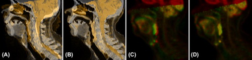
Table I. Quantitative results of the registration methods as mean (standard deviation) over all patients.
Figure 2. Map of Jacobian determinants (IJac) and corresponding deformed MR from different registration methods for Patient 1. Original CT (A), IJac from DR with GMI (B), GMI+ BEP (C) and LMI+ BEP (D). Transformed MR from RR (E), deformed MR from DR with GMI (F), GMI+ BEP (G) and LMI+ BEP (H). The structures skin and respiratory tract segmented on the original CT are shown as red contours.
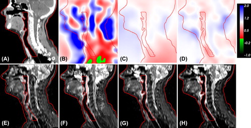
Figure 3. Axial slices of the original CT (A), transformed MR from RR (B) and from DR with LMI+ BEP (C) for Patient 2. Contours of skin (brown), bones (yellow) and respiratory tract (blue) derived from the original CT are also shown.
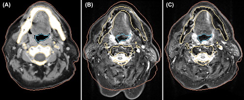
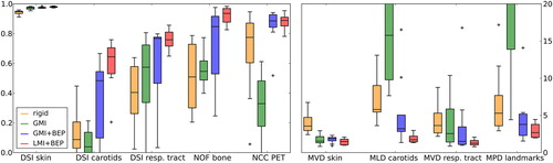
Figure 4. Quantitative results of the registration methods. Left: Boxplots of quality measures ranging between 0 and 1, with 1 being the best value. Right: Boxplots of distance quality measures, with values given in mm. Low values indicate good registration accuracy. Outliers are shown as black crosses.