Neither the SCN nor the adrenals are required for circadian time-place learning in mice

Figures & data

Table 1. Overview of experiments and groups.

Experiment	(SCN lesion Batch)	groups	N	age (months)
1. CORT		HCC	9	4
		TPL	8	4
2. LEO/FEO		HCC*	2	11
		TPL	7	11
3. SCN lesion	Batch1	HCC	8	4
		SHAM	4	4
		SCNx	5	4
	Batch2	HCC	5	4
		SHAM	4	4
		SCNx	5	4
4. Adrenalectomy	Batch2 (re-tested)	ADX	7**	7

*Not food deprived.

**3 SHAM, 4 SCNx.

The LEO/FEO experiment was performed with a separate group of animals, including TPL tested mice (TPL) and homecage control mice (HCC, not food deprived). The SCN lesion experiment was performed in two separate batches, including TPL tested SHAM- and SCN-lesioned mice. Animals with incomplete SCN lesions were not further used and are not shown. SHAM and SCNx mice from batch2 were re-tested after bilateral adrenalectomy (ADX group). In experiments 2 and 3, HCC animals were housed and food deprived together the TPL tested animals. The number of animals (N) and ages (at the beginning of TPL testing) are indicated for each group.

Figure 1. Schematic overview of the daily TPL testing protocol. Open circles indicate food (powdered standard rodent chow, <0.1 g) at the end of an arm of the maze; grey circles indicate the non-target shock location. Mice were tested individually three times a day in 10 minute trials, with an intersession time of 3 hours. Bodyweights were taken before each trial. Mice received an individual amount of food at the end of each day in order to maintain body weight at 85–87% of ad libitum feeding weight. Testing was performed in the light phase. ZT0 (zeitgeber time zero) indicates lights on.

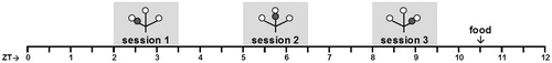
Figure 2. Phenotypic and post-mortem assessment of SCN lesions. (a–c) Sample double plotted quantitative actograms of a SHAM-lesioned mouse (a), a partial arrhythmic SCN-lesioned mouse (b), and a completely arrhythmic SCN-lesioned mouse (c), during a two week DD period. Running wheel revolutions (counted per two minute bins) are plotted with a maximum of 100 revolutions per bin. Time is marked in hours along the horizontal axis. Successive days are stacked on the vertical axis starting at the top. (d–f) Periodogram analysis of the corresponding (upper) running wheel data. A period range of 14 to 32 hours (x-axis) was analyzed with a single bin resolution. Prevalence of each period is expressed as a Qp value (y-axis). The linear grey line represents the Chi-square significance threshold (p < 0.05). Peaks extending above this threshold indicate that the corresponding period is significantly present in the data. (g–j) SCN lesion damage/extend of selected animals were verified post-mortem by silver staining. (g) Typical lesion of a TPL selected animal. Panels (h–j) summarize damage extend in all selected TPL animals. Damage extend is shown at the rostral SCN (−0.22 AP to bregma) (h), at the central SCN (−0.46 to bregma) (i) and at the caudal SCN (−0.94 to bregma) (j). The white transparent area represents maximal damage extend (area damaged in at least one animal), the dark grey transparent area represents minimal damage extend (area damaged in all TPL selected animals).

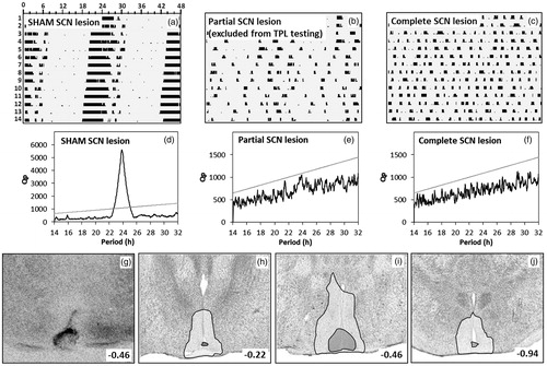
Figure 3. Average daily TPL performance after abrupt LEO and FEO phase-shifts. After testing on day 3, in the beginning of the subjective dark phase, a 3h light pulse (400–800 lux) was applied according to an Aschoff type II protocol. After performance recovered, food was delayed by 6 hours (after testing on day 8). After performance recovered, food was advanced by 6h on day 11. Days are shown on the x-axis (non-shaded days indicate testing in LD; shaded days indicate testing in DD). The grey area around the black performance curve indicates SEM. Vertical lines indicate the interventions. Chance level is indicated by the horizontal line. Daily session-specific performance is shown in bar charts underneath the average daily performance graph (x-axis days are aligned; vertical height of the bars represent relative performance).

Table 2. Post lesion rhythmicity assessment in DD.

Batch 1				Batch 2
Mouse	Visual	Period	DQp	Mouse	Visual	Period	DQp
SCN lesion
1	A	–	−217	10	A	–	−30
2	A	–	−211	11	A	–	−226
3	A	–	−162	12	A	–	−394
4	A	–	−42	13	A	–	−310
5	A	–	−289	14	A	–	−125
SHAM
6	R	23.83	3961	15	R	24.00	881
7	R	24.03	1882	16	R	23.93	804
8	R	23.80	2265	17	R	23.97	1688
9	R	23.80	4535	18	R	23.80	1609

Results from the visual and statistical rhythmicity assessment of mice selected for TPL testing. Visual assessment is based on the pattern of activity apparent in double-plotted actograms. Animals assessed as rhythmic are indicated with an ‘R’; animals assessed as arrhythmic are indicated with an ‘A’. Rhythmicity was statistically assessed by Chi-square periodogram analysis in which a period range of 14 to 32 hours was analyzed over 13 DD days. The DQp value is the difference between the Qp value and the Chi-square significance threshold. The most pronounced period (with the highest positive DQp value) is expressed in hours.

Figure 4. Spontaneous alternation (SA) results of homecage control mice (HCC, n = 13), SHAM-lesioned mice (SHAM, n = 8), SCN-lesioned mice (SCNx, n = 10) (pooled data from both batches), or mice from the second batch after adrenalectomy (ADX, n = 7). No statistical differences were found between any of the groups. Error bars represent SEM.

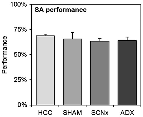
Figure 5. Habituation results and TPL learning curves. (a) Average performances of SHAM and SCNx mice during the last two habituation steps (left bar graphs) and the first 6 days of TPL testing (learning curve). (b) Combined and separate learning curves of ADX (SHAM) and ADX (SCNx) mice. Grey circular symbols represent the maze. Within, small open circles indicate food at the end of an arm of the maze and small dark grey circles indicate the application of the foot-shock. Note that only the 1st session test situations are depicted. The non-target location (non-baited and non-shock reinforced during habituation days 5–7, non-baited and shock-reinforced during habituation days 9–10, baited and shock-reinforced during actual testing on following days), changes with the TOD (i.e. session). The horizontal lines represent chance level (33%).

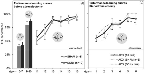
Figure 6. Baseline TPL performance and session skipping results. (a) Baseline TPL performances of the different groups when tested in the different light regimes. Baseline performance is defined as average performance on normal testing days, excluding the learning phase (first three days) and days on which manipulations (sessions skips) were performed. Batches were pooled for data from the same group and light regime. (b) Average TPL performances of the groups after multiple (different) session skips in the different light regimes. Performance was measured in the single next session after the skipped session. In both panels, chance level is indicated by the horizontal line. Error bars represent SEM. All results were significantly above chance level (# indicates p < 0.01, for unmarked bars p < 0.001).

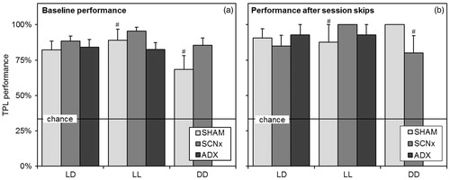
Figure 7. Corticosterone radioimmunoassay. CORT measurements were performed on animals from experiments 1 (striped bars) and 4 (black bars). Animals were sacrificed between ZT2-3.5, when animals expected to be tested in the first TPL session. Blood samples were taken from the heart prior to transcardial perfusion and CORT was measured by radioimmunoassay. Error bars represent SEM.

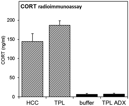
Figure 8. Representative double-plotted qualitative actograms of a SHAM SCN-lesioned mouse (a) and an SCN-lesioned mouse (b) from the second batch. TOD is plotted on the upper x-axis; days are plotted on the y-axis. Shaded areas indicate darkness. SCN lesion and adrenalectomy surgeries are indicated. Data recording failed on days 37–40. Periods in which animals were TPL tested are indicated by the dotted boxes. Within the boxes, on the right side of the actograms, grey vertical lines respectively indicate the three TPL test sessions and the time at which food was provided (thicker grey line: timed feeding/food deprivation was continued for two more days after TPL testing).

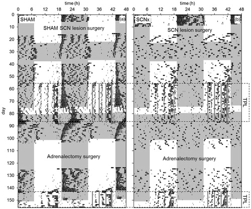
Figure 9. Activity profiles and food anticipation during TPL testing in LD. (a) Activity profile over all 30 TPL test days in LD (batch1, representative for batch 2 as well), plotted in 10 min bins. Both SHAM and SCNx mice show food anticipation. Zeitgeber time is indicated on the horizontal axis. The shaded area indicates darkness. Gray circular symbols represent the daily TPL test session situations. Within the grey circular symbols, open circles indicate food at the end of an arm of the maze, and gray circles indicate the non-target (shock) location. Horizontal error bars below the circular symbols indicate TPL test session durations. The hollow vertical arrow indicates when food was provided (daily at ZT10.5). (b) Food anticipatory activity normalized for general activity. Activity one hour before mealtime (FAA) was divided by the total daily activity (DA) minus the FAA (FAA/[DA-FAA]). No significant difference was found between SHAM and SCNx mice. In both panels, error bars represent SEM.