Figures & data
Figure 1. Illustration of the lumped parameter model from Strelioff (Citation1973).
Figure 2. Illustration of the unrolled human cochlea geometry used by Finley et al. (Citation1990). Figure a shows a close-up view of how the cross section of the cochlea and electrode is segmented; Figure b shows the full geometry.
Figure 3. Rotationally symmetric geometry of the guinea pig cochlea from Frijns et al. (Citation1995, Citation1996).
Figure 4. Spiraling tapered geometry of the implanted human cochlea from Kalkman et al. (Citation2015).
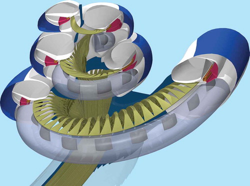
Figure 5. Schematic illustration of different multipolar strategies: bipolar stimulation (a1&a2), tripolar stimulation (b1&b2), partial tripolar stimulation with σ = 0.5 (c1&c2), and phased array stimulation for an electrode array with five contacts (d1&d2). The top figures (a1–d1) show the stimulus current amplitudes used for each multipolar strategy, and bottom figures (a2–d2) show the resulting electrical potentials along the electrode array for each individual contact (blue, red, green, purple, and orange curves), as well as their combined potential (black curve).
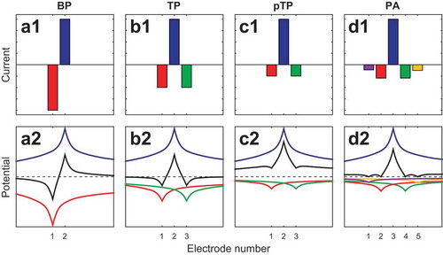
Figure 6. Schematic illustration of the current steering strategy. The curves show the electrical potential along the spiral ganglion generated by two electrode contacts, labeled E0 and E1, stimulated individually in monopolar mode (green and red dotted curves), and stimulated together as a current steered electrode pair for different values of α (blue curves). Figure a, b, and c show the potentials at α = 0.25, α = 0.5, and α = 0.75, respectively. Since the monopolar curve for E0 (green) is essentially the current steered potential for α = 0 and the curve of E1 (red) is that of α = 1, it is clear that the current steered curve (blue) gradually shifts from the monopolar field of E0 to that of E1 as the value of α increases. Note that although the peak of current steered potential is lower for intermediate values of α, this does not necessarily imply that the neural threshold is also lower.
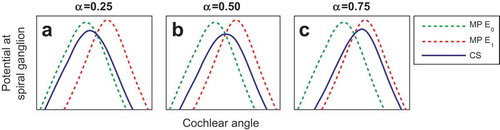
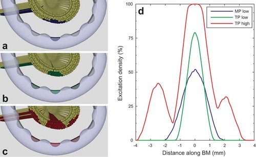
Figure 7. Illustration of excitation patterns and excitation density plots from Kalkman et al. (Citation2015). Figures a–c show neural excitation patterns in auditory neurons with degenerated peripheral processes for three different situations: (a) monopolar stimulation at low amplitude, (b) tripolar stimulation at low amplitude, exciting the same number of neurons as the monopolar stimulus above, and (c) tripolar stimulation at high amplitude. Blue, green, and red fibers in Figures a, b, and c indicate excited neurons. In Figure d, the corresponding excitation density curves are plotted, which show the percentage of neurons that are being excited along the cochlea. The blue curve corresponds to the monopolar excitation pattern shown in Figure a, the green curve to the low amplitude tripolar excitation pattern shown in Figure b, and the red curve corresponds to the excitation pattern generated by high-amplitude tripolar stimulation shown in Figure c. Comparing Figures a and b and their curves in Figure d, it is clear that tripolar stimulation excites neurons in a more spatially restricted pattern than monopolar stimulation does with the same number of excited neurons. In Figure c and the red curve in Figure d, the excitation pattern produced by a high-amplitude tripolar stimulus reveals the presence of side lobes on either side of the main excitation region, close to the flanking contacts.