From the gating charge response to pore domain movement: Initial motions of Kv1.2 dynamics under physiological voltage changes

Figures & data

Figure 1.  All-atom depiction of Kv1.2 channel double-bilayer system. The left and right boundaries are periodically connected. The K⁺ channels are represented as a purple C_α trace. The DOPC lipids (yellow) separate Bath 1 and Bath 2 displayed in pink. The chloride (green) and the potassium (blue) distribution within each bath are described in Table I. This Figure is reproduced in colour in Molecular Membrane Biology online.

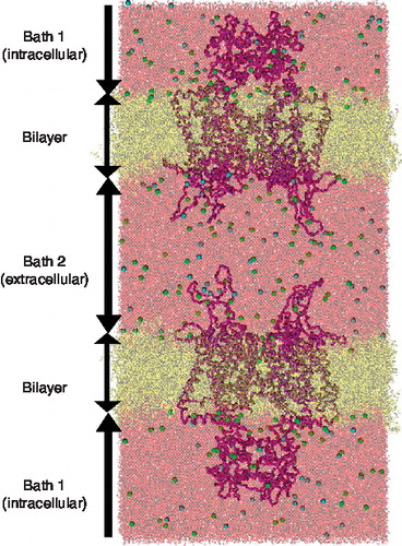
Table I.  Bath charge concentrations of the Kv1.2 channel.

System	Bath 2	Bath 1	Voltage drop
RP	694 K^+, 684 Cl^-	706 K^+, 628 Cl^-	−56 mV
DP1	695 K^+, 683 Cl^-	705 K^+, 629 Cl^-	−43 mV
DP2	696 K^+, 682 Cl^-	704 K^+, 630 Cl^-	−30 mV
DP3	697 K^+, 681 Cl^-	703 K^+, 631 Cl^-	−10 mV
DP4	698 K^+, 680 Cl^-	702 K^+, 632 Cl^-	+6 mV
DP5	699 K^+, 679 Cl^-	701 K^+, 633 Cl^-	+15 mV
Protein	147 Arg, 56 Lys, 173 Glu, 48 Asp	53 Arg, 24 Lys, 75 Glu, 72 Asp

RP = resting potential, DP = depolarized potential (The ‘protein’ contribution should be included for each system when summing each bath’s charge distribution as the residue contributions remained consistent for each bath).

Figure 2.  Establishing K⁺ channel potentials. (A) Transmembrane potential profiles at time specific averages. (Dotted line = 100 ps; dot-dashed = 1 ns; solid = 10 ns). Arrows indicate locations of bilayer. (B) Transmembrane potential profiles. The line colour corresponds to the expected voltage gradient for each system (RP = resting potential, DP = depolarized potential). The arrows along the axis indicate the location of the baths and the bilayer regions. The simulations contain a constant total number of ions. To establish the different voltage gradients ions were exchanged between the two baths. (C) The two-dimensional (xz-plane) transmembrane potential profile of the DP5 system has a 15 mV drop and shows the inhomogeneous nature of the voltage drop across the bilayer (see arrows). This Figure is reproduced in colour in Molecular Membrane Biology online.

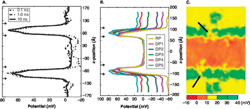
Figure 3.  The lipid hydrogen bond pattern for the individual channels as a function of voltage. (The square dot represents Arg²⁹⁴; triangle dot represents Arg²⁹⁷; diamond dot represents Arg³⁰⁰; circle dot represents Arg³⁰³) The error bars represent the standard deviation. (A) Channel 1 gating charges and the number of lipid hydrogen bonds. (B) Channel 2 gating charges and the number of lipid hydrogen bonds.

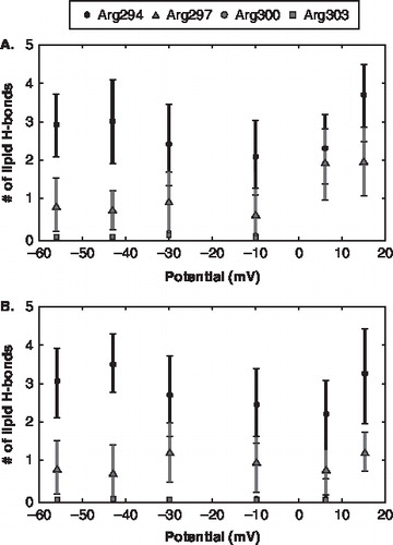
Figure 4.  Water hydrogen bonding pattern for the gating charges. The distributions show the average number of coordinating water molecules (Nij) as a function of the voltage gradient for 3 of the gating charges at different radial distribution values. (The square dot represents channel 1; the triangle dot represents channel 2). The error bars represent the standard deviation.

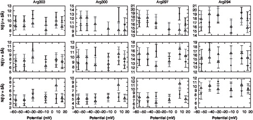
Figure 5.  The centre of mass position of the sidechain for the gating charges for each channel versus the voltage drop. The error bars represent the time-averaged standard deviation for each z-position. (The dashed line represents Arg²⁹⁴; the solid line represents Arg²⁹⁷; the dash-dot line represents Arg³⁰⁰; and a dot-dot line represents Arg³⁰³) (A) Channel 1 (B) Channel 2.

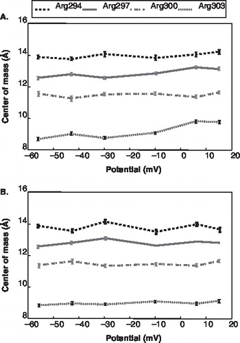
Figure 6.  The centre of mass position of the voltage sensor domain for each channel versus the voltage drop. The error bars represent the time-averaged standard deviation for each z-position. (The solid line represent channel 1; the dashed line represents channel 2) (A) S4 domain, (B) S2 domain, (C) S3 domain.

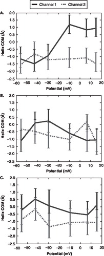
Figure 7.  The percent of displacement overlap for the pore domain as a function of mode for each voltage drop. (Yellow = RP; Pink = DP1; Cyan = DP2; Red = DP3; Green = DP4; Blue = DP5). The displacement vector represents an open ◊ closed channel vector. (A) Basic line plot (B) Natural logarithm plot (C) First 180 modes basic line plot (D) First 180 modes natural logarithm plot. This Figure is reproduced in colour in Molecular Membrane Biology online.

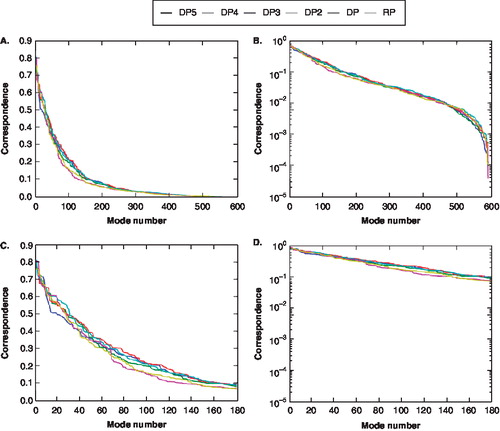
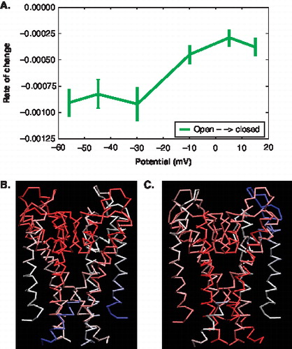
Figure 8.  Characterization of motions and displacement based on the PCA modes of the pore domain. (A) The Figure shows the rate of change in the error of overlap as a function of voltage. (represents open ◊ closed). The error bars indicate the error based on subsets of the trajectory data. (B, C) The colours indicate the degree and direction of displacement (Blue = high overlap with Δx; White = low overlap with Δx; Red = minimal overall motion) (B) C_α trace of the pore showing the motions at −56 mV. (C) C_α trace of the pore showing the motions at +15 mV. This Figure is reproduced in colour in Molecular Membrane Biology online.