A cautionary tale: The characteristics of two-dimensional distributions and their effects on epidemiological studies employing an ecological design

Figures & data

Figure 1. 1000 high-income (>2× the poverty level) earners (red) and 1000 low-income earners (blue) selected from the distributed population weighted by county-level data.

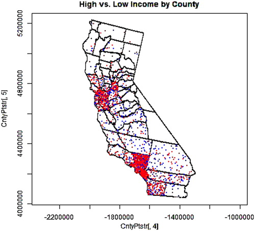
Figure 2. Two independent sets of 1000 high-income earners; one representing cases (red) and the other representing controls (blue) selected from the distributed population weighted by county-level data.

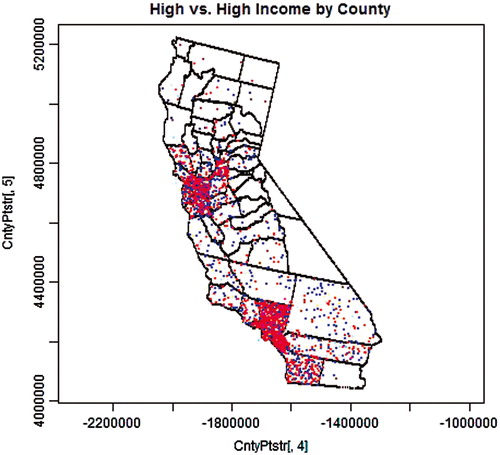
Figure 3. 1000 high-income (> 2× the poverty level) earners (red) and 1000 low-income earners (blue) selected from the distributed population weighted by census-tract-level data.

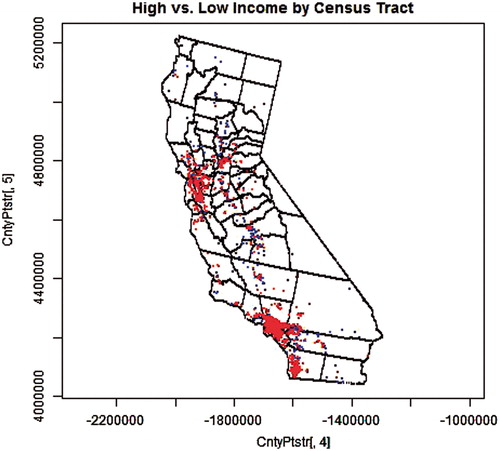
Figure 4. Two independent sets of 1000 high-income earners; one representing cases (red) and the other representing controls (blue) selected from the distributed population weighted by census-tract-level data.

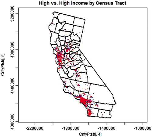
Table 1. Results of logistic regression comparing ORs for cases versus controls to proximity to ultramafic deposits in California*.

	Including data from all California counties				Excluding data from six southern California counties†
Indicated “cases” versus “controls”	OR‡	UCL¶	LCL§	P_OR||	OR‡	UCL¶	LCL§	P_OR||
Tract-level data
College degree versus no college degree	0.9648	0.9837	0.9492	1.7E−04	0.9081	0.9357	0.8786	1.5E−11
Income more than 2× poverty level versus less	0.9722	0.9921	0.9523	2.9E−03	0.9466	0.9651	0.9170	3.0E−06
White collar versus blue collar	0.9835	1.0037	0.9654	7.5E−02	0.9854	1.0075	0.9544	2.3E−01
Caucasian versus Hispanic	0.9579	0.9732	0.9387	6.2E−06	0.9466	0.9651	0.9170	3.0E−06
Caucasian versus black	0.9919	1.0070	0.9716	3.7E−01	0.9736	0.9931	0.9462	1.6E−02
Black versus Hispanic	0.9639	0.9799	0.9469	1.8E−04	0.9827	1.0062	0.9624	9.2E−02
Caucasian versus Caucasian#	1.0004	1.0162	0.9777	5.2E−01	1.0015	1.0245	0.978	5.1E−01
KS** versus pancreatic cancers**	1.0090	1.0292	0.9878	2.8E−01	0.9156	0.9415	0.8815	1.6E−10
Mesotheliomas** versus pancreatic cancers**	1.0054	1.0215	0.9884	4.4E−01	0.9984	1.018	0.9756	4.8E−01
Traffic fatalities versus pancreatic cancers**	1.0168	1.0353	0.9993	5.9E−02	1.0600	1.0887	1.0357	4.0E−07
County-level data
College degree versus no college degree	0.9752	0.9864	0.9633	1.0E−04	0.9579	0.9719	0.9388	2.4E−08
Income more than 2× poverty level versus less	0.9835	0.9969	0.9709	7.1E−03	0.9792	0.9910	0.9642	8.5E−04
White collar versus blue collar	0.9914	1.0032	0.9793	1.8E−01	1.0012	1.0145	0.9860	4.8E−01
Caucasian versus Hispanic	0.9751	0.9857	0.9619	4.1E−05	0.9691	0.9823	0.9568	3.8E−07
Caucasian versus Caucasian#	1.0001	1.0140	0.9897	5.3E−01	1.0005	1.0119	0.9868	5.2E−01
KS†† versus pancreatic cancers††	1.0031	1.0156	0.9906	4.6E−01	0.9664	0.9800	0.9485	2.2E−06
Mesotheliomas†† versus pancreatic cancers††	1.0045	1.0166	0.9913	3.3E−01	1.0006	1.0107	0.9909	4.7E−01
Traffic fatalities versus pancreatic cancers††	1.0153	1.0275	1.0032	6.6E−03	1.0247	1.0388	1.0129	4.4E−05

*The natural logs of the odds ratios for cases versus controls were regressed against proximity to ultramafic rocks. In each regression, street-address level locations for cases and controls were separately chosen at random within each county (or census tract) with numbers proportional to their respective population within that county (or census tract). A total of 1000 each of cases and controls were selected statewide during each iteration. Results represent the 50th percentiles of 200 independent regressions. UCLs and LCLs respectively represent the 97.5th and 2.5th percentiles of the resulting OR's.

†The six southern California counties eliminated are: Imperial, Los Angeles, Orange, Riverside, San Diego and Ventura. These were eliminated because they contain virtually no ultramafic deposits.

‡This is the OR at standard distance for the indicated association. It is the exponential of the regression coefficient and can be interpreted to represent the fractional decrease (or increase, if greater than one) in “risk” with every 10 km increase in distance. Regressions were scaled to 10 km distances in this study so that the magnitude of the coefficients would be directly comparable to those reported by Pan et al. (2005). Boxed values show larger effects than those reported by Pan et al.

¶This is the two-tailed 95% upper confidence limit on the OR.

§This is the two-tailed 95% lower confidence limit on the OR.

||This is the p value for the OR (and the corresponding regression coefficient). By convention, values of 0.05 or less are considered significant and are therefore bolded and italicized.

#Caucasians versus Caucasians represent regressions in which the locations of cases and controls were derived from the same marginal distribution (Caucasians) so that any “non-uniform” heterogeneity (defined in the accompanying text) between cases and controls is eliminated. Thus, these runs serve as negative controls because no effect is expected.

**Cases and controls for cancers are based on sampling the distribution of estimated cancers derived as the product of the (annualized) age-adjusted rate per 100 000 in the indicated county multiplied by the at-risk population in the corresponding county (divided by 100 000). County data were then extrapolated to tract-level data by obtaining counts for individual ethnic groups as the product of the county-rate and the tract-level population of each ethnicity and summing over ethnic groups.

††Numbers of countywide cases and controls were derived as described in the previous footnote.

Table 2. Estimates of ORs, intercepts and frequencies for cases versus controls regressed against sets of random sources (county-level data)*.

Cases	Controls	OR†	LTail‡ OR	UTail¶ OR	Fraction significant (%)§	Fraction steeper (%)||	Fraction increasing (%)#	Fraction decreasing (%)**	Intercept	LTail‡ intercept	UTail¶ intercept	Fraction significant (%)††
County-level data from all counties in California
Caucasians	Hispanics	0.9898	0.7279	1.3539	10	68	47	53	1.0065	0.8259	1.2301	7
Caucasians‡‡	Caucasians‡‡	1.0025	0.7754	1.2914	5	62	51	49	0.9984	0.8496	1.1758	3
Caucasians	Blacks	1.1464	0.5499	2.5840	56	89	62	38	0.9179	0.5675	1.5046	51
Blacks	Hispanics	0.8612	0.3824	1.8714	56	89	36	64	1.0983	0.6554	1.7891	51
White collar workers	Blue collar workers	1.0066	0.7708	1.3071	5	63	52	48	0.9958	0.8433	1.1799	3
College graduates	Non-college graduates	1.0161	0.7657	1.3417	7	65	54	46	0.9899	0.8281	1.1836	4
Income > twice poverty level	Income ≤ twice poverty level	1.0098	0.7636	1.3252	7	65	53	47	0.9938	0.8361	1.1881	4
Mesotheliomas	Pancreatic cancers	1.0109	0.7750	1.3168	5	62	54	46	0.9932	0.8421	1.1745	3
KS	Pancreatic cancers	0.9603	0.6600	1.4725	21	77	42	58	1.0260	0.7730	1.2852	16
Traffic deaths	Pancreatic cancers	0.9946	0.7493	1.3515	8	66	48	52	1.0034	0.8301	1.2062	5
County-level data excluding six counties in southern California¶¶
Caucasians	Hispanics	1.0106	0.7517	1.3348	7	66	53	47	0.9933	0.8324	1.1937	4
Caucasians‡‡	Caucasians‡‡	1.0003	0.7683	1.3042	5	63	50	50	0.9998	0.8459	1.1823	3
Caucasians	Blacks	1.2455	0.3217	5.8225	72	93	62	38	0.8720	0.3848	2.2568	68
Blacks	Hispanics	0.8160	0.1659	3.1830	70	93	38	62	1.1356	0.4367	2.6386	67
White collar workers	Blue collar workers	1.0098	0.7697	1.3245	6	64	53	47	0.9940	0.8362	1.1766	3
College graduates	Non-college graduates	1.0195	0.7287	1.4067	12	70	55	45	0.9879	0.8014	1.2156	8
Income > twice poverty level	Income ≤ twice poverty level	1.0179	0.7539	1.3554	8	67	55	45	0.9888	0.8234	1.1908	5
Mesotheliomas	Pancreatic cancers	1.0127	0.7689	1.3354	6	65	54	46	0.9920	0.8344	1.1810	3
KS	Pancreatic cancers	0.8784	0.5022	2.0835	59	91	39	61	1.0843	0.6059	1.5078	54
Traffic deaths	Pancreatic cancers	0.9945	0.7380	1.3491	9	68	49	51	1.0036	0.8293	1.2148	5

*The natural logs of the ORs for cases versus controls were regressed against proximity to sets of (2500) random locations. In each regression, street-address level locations for cases and controls were separately chosen at random within each county with numbers proportional to their respective population within that county. A total of 1000 each of cases and controls were selected state-wide during each iteration. OR results represent the 50th percentile of 10 000 regressions grouped as 200 sets of cases and controls regressed against each of 50 independent sets of (2500) random locations.

†This is the OR at standard distance for the association. It is the exponential of the regression coefficient and can be interpreted to represent the fractional decrease (or increase if greater than one) in “risk” with every 10 km increase in distance. Regressions were scaled to 10 km distances in this study so that the magnitude of the coefficients would be directly comparable to those reported by Pan et al. (2005).

‡This is the lower tail (2.5th percentile) of the distribution of OR's observed across all (50 × 200 = 10 000) regressions.

¶This is the upper tail (97.5th percentile) of the distribution of OR's observed across all (50 × 200 = 10 000) regressions.

§This is the fraction of regressions (200 × 50 = 10 000) for which the OR (and, correspondingly, the regression coefficient) was observed to be significant.

||This is the fraction of regressions for which a greater absolute OR (i.e. < 0.937 or >1.067) is observed than that reported by Pan et al. 2005. Note that 1.067 is the reciprocal of 0.937, which simply represents an increasing (rather than decreasing) trend.

#This is the fraction of regressions for which an OR greater than 1 is observed, which is equivalent to a positive regression coefficient and means that the number of cases increases with distance from putative sources.

**This is the fraction of regressions for which an OR less than 1 is observed, which is equivalent to a negative regression coefficient and means that the number of cases decreases with distance from putative sources.

††This is the fraction of regressions for which the intercept was observed to be significant.

‡‡Caucasians versus Caucasians represent regressions in which the locations of cases and controls were derived from the same marginal distribution (Caucasians), so that any “non-uniform” heterogeneity (defined in the text accompanying Table 1) between cases and controls is eliminated. Thus, these runs which are highlighted, serve as negative controls because no effect is expected.

¶¶Counties excluded from these analyses are: Imperial, Los Angeles, Orange, Riverside, San Diego and Ventura.

Table 3. Estimates of ORs, intercepts and frequencies for cases versus controls regressed against distance to random sources (tract-level data)*.

Cases	Controls	OR†	LTail‡ OR	UTail¶ OR	Fraction significant (%)§	Fraction steeper (%)||	Fraction increasing (%)#	Fraction decreasing (%)**	Intercept	LTail‡ intercept	UTail¶ intercept	Fraction significant (%)††
Tract-level data from all counties in California
Caucasians	Hispanics	0.9527	0.4773	1.6084	33	79	42	58	1.0311	0.7506	1.6364	26
Caucasians‡‡	Caucasians‡‡	1.0040	0.7749	1.3065	5	61	52	48	0.9975	0.8456	1.1740	3
Caucasians	Blacks	0.9517	0.3456	2.2278	62	89	46	54	1.0325	0.6275	2.0954	58
Blacks	Hispanics	1.0913	0.3816	2.7705	58	92	57	43	0.9470	0.4813	1.7699	52
White collar workers	Blue collar workers	0.9810	0.7152	1.3476	11	68	45	55	1.0120	0.8295	1.2346	7
College graduates	Non-college graduates	0.9737	0.6611	1.4354	19	74	45	55	1.0171	0.7926	1.2945	14
Income > twice poverty level	Income ≤ twice poverty level	0.9793	0.6345	1.4587	21	74	46	54	1.0131	0.7885	1.3492	15
Mesotheliomas¶¶	Pancreatic cancers¶¶	1.0012	0.7571	1.3163	6	64	50	50	0.9993	0.8428	1.1866	3
KS¶¶	Pancreatic cancers¶¶	0.9549	0.5963	1.6738	32	81	43	57	1.0292	0.7089	1.3583	26
Traffic fatailities¶¶	Pancreatic cancers¶¶	1.0091	0.7235	1.4144	12	70	52	48	0.9945	0.8100	1.2285	8
Tract-level data excluding six counties in southern Californial
Caucasians	Hispanics	0.9108	0.5657	1.4699	28	79	33	67	1.0601	0.7872	1.4563	23
Caucasians‡‡	Caucasians‡‡	0.9967	0.7586	1.3087	5	64	49	51	1.0021	0.8428	1.1859	3
Caucasians	Blacks	0.9567	0.3895	2.5858	54	87	45	55	1.0283	0.5811	1.9604	51
Blacks	Hispanics	0.9808	0.3523	2.5632	47	85	48	52	1.0121	0.5057	1.8618	43
White collar workers	Blue collar workers	1.0075	0.6886	1.3978	13	71	51	49	0.9953	0.8090	1.2517	8
College graduates	Non-college graduates	0.9705	0.5764	1.4403	21	75	44	56	1.0187	0.7862	1.3788	17
Income > twice poverty level	Income ≤ twice poverty level	1.0110	0.6567	1.6264	29	82	51	49	0.9932	0.7345	1.3039	23
Mesotheliomas¶¶	Pancreatic cancers¶¶	1.0021	0.7442	1.3400	7	66	51	49	0.9987	0.8346	1.2012	4
KS¶¶	Pancreatic cancers¶¶	0.7896	0.4068	2.9863	68	92	31	69	1.1519	0.4549	1.6705	64
Traffic Fatailities¶¶	Pancreatic cancers¶¶	1.0217	0.6679	1.4476	14	73	55	45	0.9870	0.7953	1.2883	10

*The natural logs of the ORs for cases versus controls were regressed against proximity to sets of (2500) random locations. In each regression, street-address level locations for cases and controls were separately chosen at random within each census tract with numbers proportional to their respective population within that census tract. A total of 1000 each of cases and controls were selected statewide during each iteration. OR results represent the 50th percentile of 5400 regressions grouped as 200 sets of cases and controls regressed against each of 27 independent sets of (2500) random locations (unless otherwise indicated; see Footnote ¶¶).

†This is the OR at standard distance for the association. It is the exponential of the regression coefficient and can be interpreted to represent the fractional decrease (or increase if greater than one) in “risk” with every 10 km increase in distance. Regressions were scaled to 10 km distances in this study so that the magnitude of the coefficients would be directly comparable to those reported by Pan et al. (2005).

‡This is the lower tail (2.5th percentile) of the distribution of OR's observed across all regressions.

¶This is the upper tail (97.5th percentile) of the distribution of OR's observed across all regressions (either 5400 or 10 000 depending on the population; see Footnote ¶¶).

§This is the fraction of regressions (200 × 27 = 5400 or 200 × 50 = 10 000 for indicated populations, see Footnote ¶¶) for which the OR was observed to be significant.

||This is the fraction of regressions for which a greater absolute OR (i.e. < 0.937 or >1.067) is observed than that reported by Pan et al. (2005). Note that 1.067 is the reciprocal of 0.937, which simply represents an increasing (rather than decreasing) trend.

#This is the fraction of regressions for which an OR greater than 1 is observed, meaning that the number of cases increases with distance from target locations (putative sources).

**This is the fraction of regressions for which an OR less than 1 is observed, meaning that the number of cases decreases with distance from target locations (putative sources).

††This is the fraction of regressions for which the intercept was observed to be significant.

‡‡Caucasians versus Caucasians represent regressions in which the locations of cases and controls were derived from the same marginal distribution (Caucasians) so that any “non-uniform” heterogeneity (defined in the text accompanying Table 1) between cases and controls is eliminated. Thus, these runs which are highlighted, serve as negative controls because no effect is expected.

¶¶Regressed against each of 50 independent sets of 2500 random locations chosen within the State of California.

§§Counties excluded from these analyses are: Imperial, Los Angeles, Orange, Riverside, San Diego and Ventura.

Table 4. Results from simulating the distribution of population characteristics within census tracts to evaluate associations with proximity to ultramafic rock*.

Assumed slopes/OR's†		Cases have college degree controls don't‡					Cases have > 2 × poverty level Income controls don't‡					Cases are white collar controls are blue collar¶
OR	Slope§	Observed OR||	Observed slope§	OR UCL95#	OR LCL95**	p Value††	Observed OR||	Observed slope§	OR UCL95#	OR LCL95**	p Value††	Observed OR||	Observed slope§	OR UCL95#	OR LCL95**	p Value††
Casesadj versus Controls
1	0	0.916	−0.088	0.941	0.890	1.9E−11	0.950	−0.051	0.971	0.928	7.1E−07	0.982	−0.018	1.001	0.964	9.2E−02
0.937	−0.065	0.911	−0.094	0.935	0.877	1.3E−16	0.941	−0.061	0.963	0.919	5.6E−11	0.976	−0.025	0.996	0.953	1.5E−02
0.771	−0.260	0.891	−0.116	0.913	0.860	3.1E−20	0.921	−0.082	0.941	0.896	9.1E−16	0.958	−0.043	0.979	0.933	1.0E−04
0.353	−1.041	0.794	−0.231	0.830	0.748	1.6E−31	0.832	−0.184	0.866	0.799	3.8E−30	0.880	−0.128	0.905	0.843	3.9E−15
Controls versus Casesadj
1	0	1.091	0.087	1.130	1.067	1.6E−11	1.054	0.053	1.078	1.030	3.2E−07	1.018	0.018	1.038	0.999	9.2E−02
0.937	−0.065	1.087	0.084	1.121	1.057	2.5E−11	1.047	0.046	1.074	1.022	4.0E−06	0.948	−0.054	0.976	0.919	3.0E−06
0.771	−0.260	1.069	0.067	1.103	1.040	2.3E−07	1.028	0.027	1.056	1.007	7.1E−03	0.931	−0.072	0.962	0.906	5.8E−09
0.353	−1.041	0.999	−0.002	1.027	0.969	4.6E−01	0.963	−0.037	0.988	0.940	2.2E−03	0.880	−0.128	0.905	0.843	3.9E−15
Casesadj versus Cases
1	0	1.000	0.000	1.029	0.976	5.3E−01	1.001	0.001	1.021	0.976	4.8E−01	1.001	0.001	1.020	0.977	4.8E−01
0.937	−0.065	0.993	−0.007	1.020	0.963	3.9E−01	0.992	−0.008	1.015	0.972	3.1E−01	0.994	−0.006	1.005	0.977	6.1E−01
0.771	−0.260	0.975	−0.026	0.994	0.952	6.4E−03	0.972	−0.028	0.996	0.951	7.8E−03	0.976	−0.025	0.987	0.963	5.9E−02
0.353	−1.041	0.903	−0.103	0.934	0.865	5.0E−09	0.901	−0.105	0.933	0.875	7.0E−13	0.904	−0.101	0.921	0.885	1.2E−09

*Results of logistic regression of Cases_adj versus Controls, Controls versus Cases_adj or Cases_adj versus Cases with closest distance to ultramafic deposits as the independent variable. In each regression, street-address level locations for controls were separately chosen at random within each census tract with numbers proportional to their population within that census tract. Case_adj locations were similarly chosen at random, but with numbers proportional to a population within each census tract estimated (with binomial variation) as the product of the assumed OR and the number of unadjusted cases in that census tract. A total of 1000 each of cases and controls were selected statewide during each iteration. For all of the analyses presented, populations in Imperial, Los Angeles, Orange, Riverside, San Diego and Ventura Counties were excluded from the calculations.

†These are the (assumed) OR at standard distance and the corresponding slopes used to calculate the populations of adjusted cases whose relative distances to ultramafics were compared to the indicated, second population using logistic regression. As detailed in the Methods section (and Footnote * above), estimated populations were also calculated by incorporating binomial variation about their expectation value.

‡Results based on 200 iterations.

¶Results based on 100 iterations.

§These highlighted columns show the regression (slope) coefficients corresponding to the odds ratios presented in the previous columns. In logistic regression, the exponential of the slope coefficients represent the odds ratios at standard distance between cases and controls. Nevertheless, typically, it is the OR's themselves that are reported in studies employing logistic regression.

||These are the observed OR's for the association between the indicated characteristic and the distance to ultramafic rock. Values less than one indicate that the population of cases decreases relative to controls as distance from ultramafic rock increases. Values greater than one indicate that cases increase relative to controls at increasing distance.

#These upper confidence bounds represent the 97.5th percentile of the observed distribution of observed OR's over the indicated number of iterations.

**These lower confidence bounds represent the 2.5th percentile of the observed distribution of observed OR's over the indicated number of iterations.

††These p values indicate the significance of the test of whether the observed OR's differs from one (and, correspondingly, whether the regression coefficient differs from zero). Significant values are bolded.

Table 5. Observed ratios of “Cases” versus “Controls” for indicated characteristics among the 7049 census tracts and 58 counties in California*.

Ratios: cases to controls		Fraction of observed ratios at least as extreme as indicated ratios
Relative	Absolute	Reciprocal	Higher versus lower income (%)†	College degree versus none (%)	White collar versus blue collar (%)	Caucasians versus Hispanics (%)	Caucasians versus blacks (%)	Mesothelioma versus pancreatic (%)	KS versus pancreatic (%)	Traffic deaths versus pancreatic (%)
Census tract data
	0.1	10.00	3	6	7	21	27	0	0	0
	0.2	5.00	15	19	17	40	45	0	3	0
	0.3	3.33	31	33	28	55	58	0	13	0
	0.4	2.50	44	47	38	66	67	0	20	2
	0.5	2.00	57	59	49	74	74	0	25	10
	0.6	1.67	67	69	60	81	81	1	38	32
	0.7	1.43	76	78	70	87	86	4	72	78
	0.8	1.25	85	86	81	92	91	23	84	85
80/20	0.25	4	23	26	22	49	52	0	7	0
75/25	0.33	3	35	37	31	59	61	0	14	1
70/30	0.43	2.33	48	50	41	68	69	0	20	2
60/40	0.67	1.5	73	75	67	85	85	2	43	47
50/50	1.00	1	99	100	100	100	100	100	100	100
County data
	0.1	10.00	0	0	0	9	33	3	5	0
	0.2	5.00	0	0	0	28	47	3	12	3
	0.3	3.33	0	0	3	40	59	3	26	9
	0.4	2.50	3	24	7	50	66	7	38	29
	0.5	2.00	12	33	16	57	74	7	43	47
	0.6	1.67	29	59	24	66	76	14	50	66
	0.7	1.43	53	67	38	81	81	22	55	78
	0.8	1.25	67	72	64	90	88	47	62	90
80/20	0.25	4	0	0	0	34	55	3	17	3
75/25	0.33	3	0	7	5	43	62	3	29	12
70/30	0.43	2.33	5	24	10	50	66	7	38	29
60/40	0.67	1.5	47	59	33	76	79	16	52	72
50/50	1.00	1	100	100	100	100	100	100	100	100

*Each cell of this table represents the fraction of counties (or census tracts) in which the ratio of cases to controls (or controls to cases) is more extreme than the indicated ratio. Thus, for example, “24%” in the fifth column of the shaded row near the bottom of the table representing a ratio of 70/30 (70% to 30%) in the column for College degrees versus none (cases being those with a college degree and controls having no degree) indicates that 24% of California Counties show ratios of cases versus controls (or controls versus cases) of 70/30 or more extreme for these populations. Highlighted rows represent ratios equal to or bracketing a ratio of 70/30. Percentages of geographic units exceeding indicated “case/control” ratios that are greater than 50% are bolded

†This is the number of individuals with an income that is twice the poverty level versus less.

Figure 5. 1000 Cases (red) and 1000 Controls (blue) sampled from a set of 500 simulated “municipalities” of randomly varying sizes and locations with a randomly selected half weighted to favor cases (70%/30%) and the other half favoring controls (70%/30%).

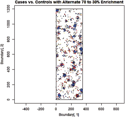
Figure 6. 1000 Cases (red) and 1000 Controls (blue) sampled from a set of 500 simulated “municipalities” of randomly varying sizes and locations with each weighted equally (50%/50%), neither favoring cases or controls.

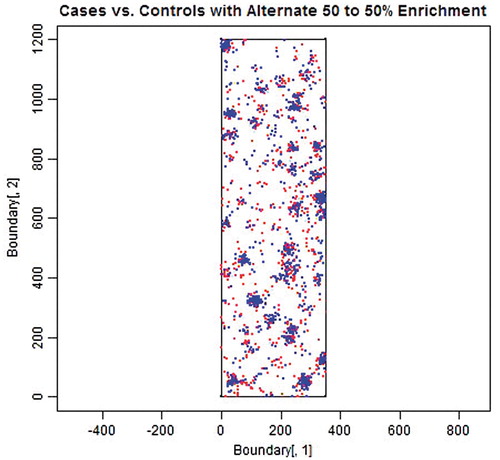
Table 6. Summary results of four sets of 2500 regressions conducted to test a hypothetical mechanism underlying the excessive numbers of false-positive (non-causal) associations observed among California demographic data*.

Degree of Enrichment†	OR‡	LTail¶ OR	UTail§ OR	Fraction significant (%)||	Fraction steeper (%)#	Fraction increasing (%)**	Fraction decreasing (%)††	Intercept	LTail¶ intercept	UTail§ intercept	Fraction significant (%)‡‡
50–50%	1.0011	0.7773	1.2884	5	63	50	50	0.9992	0.8472	1.1801	3
70–30%	0.9935	0.7260	1.3865	13	71	48	52	1.0043	0.8066	1.2360	9
75–25%	1.0044	0.6937	1.4440	17	72	51	49	0.9971	0.7836	1.2732	13
80–20%	0.9985	0.6711	1.5048	22	74	50	50	1.0010	0.7668	1.2972	17

*Based on 50 realizations of 1000 cases and 1000 controls regressed against each of 50 independent sets of 2500 random locations chosen within a rectangle representing a “stylized” California. Cases and controls were each located by a stratified random mechanism described in the “mechanism discussion” of the “Methods” section of the text. A total of 2500 regressions (50 realizations × 50 sets) were completed overall.

†This is the relative fraction of cases versus controls in each of 500 simulated municipalities of varying sizes randomly located across a stylized State of California.

‡This is the median of 2500 estimates of the OR at standard distance (which is the exponential of the regression coefficient) for the association. It can be interpreted to represent the fractional decrease (or increase if greater than one) in “risk” with every 10 km increase in distance. Regressions were scaled to 10 km distances in this study so that the magnitude of the coefficients would be directly comparable to those reported by Pan et al. (2005).

¶This is the lower tail (2.5th percentile) of the distribution of OR's (or intercepts) observed across all 2500 regressions.

§This is the upper tail (97.5th percentile) of the distribution of OR's (or intercepts) observed across all 2500 regressions.

||This is the fraction of the 2500 regressions for which the OR (and correspondingly the regression coefficient) was observed to be significant.

#This is the fraction of regressions for which a greater absolute OR (i.e. < 0.937 or >1.067) is observed than that reported by Pan et al. (2005). Note that 1.067 is the reciprocal of 0.937, which simply represents an increasing (rather than decreasing) trend.

**This is the fraction of regressions for which an OR greater than 1 is observed, which is equivalent to a positive regression coefficient and means that the number of cases increases with distance from putative sources.

††This is the fraction of regressions for which an OR less than 1 is observed, which is equivalent to a negative regression coefficient and means that the number of cases decreases with distance from putative sources.

‡‡This is the fraction of the 2500 regressions for which the intercept was observed to be significant.

Table 7. Distribution of results from sets of regressions conducted to test a hypothetical mechanism underlying the excessive numbers of false-positive associations observed among California demographic data*.

Percentiles†	OR‡	Ltail¶ OR	Utail§ OR	Fraction significant (%)||	Fraction steeper (%)#	Fraction increasing (%)**	Fraction decreasing (%)††	intercept	Ltail¶ intercept	UTail§ intercept	Fraction significant (%)††
Percentiles of 50 iterations of 50 regressions each (assumed: 50–50% – no enrichment among cases and controls)
Min	0.9556	0.6405	1.2031	0	50	36	40	0.9764	0.7826	1.1185	0
5th%ile	0.9767	0.6976	1.2261	0	54	42	43	0.9830	0.7978	1.1300	0
10th%ile	0.9814	0.7194	1.2321	2	54	44	44	0.9855	0.8082	1.1376	0
20th%ile	0.9876	0.7289	1.2519	2	58	46	46	0.9910	0.8236	1.1445	0
50th%ile	1.0032	0.7736	1.2908	4	62	52	48	0.9979	0.8477	1.1801	2
80th%ile	1.0142	0.8107	1.3491	6	68	54	54	1.0084	0.8639	1.2261	4
90th%ile	1.0225	0.8203	1.3716	8	72	56	56	1.0120	0.8720	1.2428	6
95th%ile	1.0268	0.8289	1.4134	9	72	57	58	1.0152	0.8735	1.2646	6
Max	1.0366	0.8419	1.4599	12	78	60	64	1.0303	0.8876	1.3340	8
Percentiles of 50 iterations of 50 regressions each (assumed: 70–30% enrichment of cases or controls among 500 municipalities)
Min	0.9010	0.6171	1.2524	2	54	32	32	0.9496	0.7275	1.1511	2
5th%ile	0.9345	0.6416	1.3022	6	60	34	37	0.9695	0.7522	1.1745	2
10th%ile	0.9436	0.6539	1.3127	8	60	40	40	0.9768	0.7648	1.1905	4
20th%ile	0.9591	0.6870	1.3376	10	62	40	46	0.9855	0.7790	1.2116	6
50th%ile	0.9985	0.7177	1.4067	14	72	50	50	1.0010	0.7998	1.2412	8
80th%ile	1.0226	0.7468	1.4619	18	76	54	60	1.0272	0.8279	1.2742	12
90th%ile	1.0348	0.7667	1.4986	18	80	60	60	1.0376	0.8374	1.3162	14
95th%ile	1.0475	0.7806	1.5429	20	82	63	66	1.0446	0.8434	1.3393	17
Max	1.0846	0.8072	1.6218	24	92	68	68	1.0728	0.8651	1.3829	22
Percentiles of 50 iterations of 50 regressions each (assumed: 75–25% enrichment)
Min	0.9455	0.5836	1.3153	4	54	28	30	0.9552	0.6926	1.1253	2
5th%ile	0.9510	0.6095	1.3329	10	64	40	37	0.9681	0.7126	1.1737	7
10th%ile	0.9590	0.6332	1.3621	12	66	42	40	0.9702	0.7332	1.2230	8
20th%ile	0.9811	0.6528	1.3846	14	66	44	42	0.9819	0.7499	1.2342	8
50th%ile	1.0037	0.6852	1.4559	17	72	51	49	0.9975	0.7800	1.2822	12
80th%ile	1.0280	0.7218	1.5438	20	78	58	56	1.0124	0.8090	1.3339	16
90th%ile	1.0471	0.7383	1.6075	24	80	60	58	1.0278	0.8183	1.3533	18
95th%ile	1.0504	0.7851	1.6681	26	80	63	60	1.0332	0.8295	1.3849	20
Max	1.0705	0.8317	1.7424	28	82	70	72	1.0363	0.8354	1.4293	26
Percentiles of 50 iterations of 50 regressions each (assumed: 80–20% enrichment)
Min	0.9449	0.5331	1.3637	10	58	38	36	0.9301	0.6922	1.1945	8
5th%ile	0.9518	0.5815	1.3798	13	66	40	38	0.9658	0.7057	1.2231	10
10th%ile	0.9612	0.6124	1.4092	16	68	42	40	0.9736	0.7111	1.2364	12
20th%ile	0.9658	0.6233	1.4535	16	68	44	44	0.9832	0.7328	1.2644	12
50th%ile	0.9966	0.6660	1.5114	22	74	50	50	1.0023	0.7620	1.3090	16
80th%ile	1.0260	0.7011	1.6064	26	80	56	56	1.0225	0.7830	1.3641	20
90th%ile	1.0427	0.7182	1.6721	30	80	60	58	1.0259	0.7992	1.3797	22
95th%ile	1.0555	0.7382	1.6944	32	82	62	60	1.0333	0.8117	1.4059	23
Max	1.1186	0.7632	1.7728	40	86	64	62	1.0378	0.8169	1.4923	40

*Based on 50 realizations of 1000 cases and 1000 controls regressed against each of 50 independent sets of 2500 random locations chosen within a rectangle representing a “stylized” California. Cases and controls were each located by a stratified random mechanism described in the “mechanism discussion” of the Methods Section of the text. A total of 2500 regressions (50 realizations × 50 sets) were completed overall.

†These are the percentiles of the distributions of the indicated factors observed across 50 sets of regressions. Median values are highlighted. Each of the 50 sets contains 50 independent realizations of 1000 randomly generated cases and controls with the natural log of their odds ratios regressed against nearest distance to a particular set of 2500 putative sources. A different (randomly selected) set of sources was generated for each of the 50 sets of regressions.

‡This is the OR at standard distance (which is the exponential of the regression coefficient) for the association. It can be interpreted to represent the fractional decrease (or increase if greater than one) in “risk” with every 10 km increase in distance. Regressions were scaled to 10 km distances in this study so that the magnitude of the coefficients would be directly comparable to those reported by Pan et al. (2005).

¶This is the lower tail (2.5th percentile) of the distribution of OR's (or intercepts) observed across the 50 regressions (each incorporating a unique realization of locations for cases and controls) within a single set. The percentiles reported for the tails in the table are observed across the 50 sets (each set incorporating a distinct set of hypothetical sources).

§This is the upper tail (97.5th percentile) of the distribution of OR's (or intercepts) observed across the 50 regressions (each incorporating a unique realization of locations for cases and controls) within a single set. The percentiles reported for the tails in the table are observed across the 50 sets (each set incorporating a distinct set of hypothetical sources).

||This is the fraction of the 2500 regressions for which the OR (and correspondingly the regression coefficient) was observed to be significant.

#This is the fraction of regressions for which a greater absolute OR (i.e. < 0.937 or >1.067) is observed than that reported by Pan et al. (2005). Note that 1.067 is the reciprocal of 0.937, which simply represents an increasing (rather than decreasing) trend.

**This is the fraction of regressions for which an OR greater than 1 is observed, which is equivalent to a positive regression coefficient and means that the number of cases increases with distance from putative sources.

††This is the fraction of regressions for which an OR less than 1 is observed, which is equivalent to a negative regression coefficient and means that the number of cases decreases with distance from putative sources.

‡‡This is the fraction of the 50 regressions from each set for which the intercept was observed to be significant.

Figure 7. 2500 source locations uniformly distributed around the stylized state.

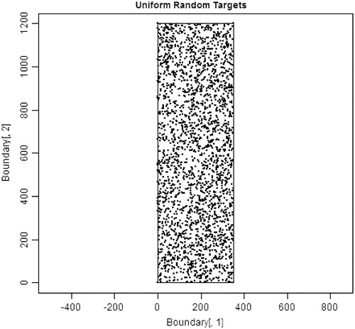
Figure 8. 100 source locations distributed non-uniformly along two vertical lines that are each 50 km inward from the north-south boundaries of the stylized state. Note that the number of locations was reduced from 2500, so that the random nature of the distribution along each vertical line could be easily observed.

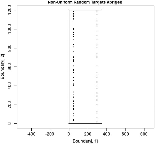
Table 8. Distribution of results from sets of regressions conducted to test a hypothetical mechanism underlying the excessive numbers of false-positive associations observed among California demographic data and highly non-uniform target locations*.

Percentiles†	OR‡	Ltail¶ OR	Utail§ OR	Fraction significant (%)||	Fraction steeper (%)#	Fraction increasing (%)**	Fraction decreasing (%)††	Intercept	Ltail¶ intercept	UTail§ intercept	Fraction significant (%)‡‡
Percentiles of 50 iterations of 50 regressions each (assumed: 50–50% – no enrichment)
Min	0.9950	0.9651	1.0164	0	0	36	36	0.9816	0.8343	1.0738	0
5th%ile	0.9965	0.9684	1.0188	0	0	40	41	0.9843	0.8456	1.0944	0
10th%ile	0.9969	0.9706	1.0197	2	0	42	42	0.9890	0.8535	1.1070	0
50th%ile	1.0002	0.9756	1.0242	4	0	50	50	0.9991	0.8821	1.1386	0
90th%ile	1.0021	0.9808	1.0308	8	0	58	58	1.0149	0.9032	1.1733	4
95th%ile	1.0031	0.9829	1.0318	9	0	59	60	1.0192	0.9079	1.1858	4
Max	1.0038	0.9860	1.0361	16	0	64	64	1.0249	0.9137	1.2262	6
Percentiles of 50 iterations of 50 regressions each (assumed: 60–40% enrichment)
Min	0.9928	0.9492	1.0209	6	0	34	34	0.9667	0.7620	1.1465	2
5th%ile	0.9940	0.9518	1.0251	10	0	36	37	0.9730	0.7777	1.1527	4
10th%ile	0.9953	0.9536	1.0265	10	0	40	40	0.9810	0.7814	1.1620	4
50th%ile	0.9990	0.9649	1.0373	18	0	48	52	1.0049	0.8298	1.2056	10
90th%ile	1.0038	0.9709	1.0472	24	0	60	60	1.0257	0.8682	1.3043	16
95th%ile	1.0049	0.9712	1.0515	27	0	63	64	1.0311	0.8781	1.3171	17
Max	1.0063	0.9736	1.0534	32	0	66	66	1.0356	0.8927	1.3606	20
Percentiles of 50 iterations of 50 regressions each (assumed: 70–30% enrichment)
Min	0.9896	0.9260	1.0359	26	0	32	32	0.9453	0.6565	1.1975	18
5th%ile	0.9927	0.9280	1.0427	30	0	38	38	0.9503	0.6770	1.2650	22
10th%ile	0.9933	0.9307	1.0471	34	0	40	42	0.9690	0.6851	1.2766	24
50th%ile	1.0006	0.9434	1.0592	42	2	50	50	0.9971	0.7350	1.3604	30
90th%ile	1.0066	0.9551	1.0760	52	6	58	60	1.0337	0.7857	1.4438	40
95th%ile	1.0098	0.9564	1.0802	52	6	62	62	1.0368	0.8039	1.4969	41
Max	1.0107	0.9622	1.0858	60	12	68	68	1.0580	0.8163	1.5129	44
Percentiles of 50 iterations of 50 regressions each (assumed: 75–25% enrichment)
Min	0.9900	0.9204	1.0677	42	2	38	46	0.9773	0.5901	1.3625	36
5th%ile	0.9917	0.9223	1.0724	44	4	40	48	0.9824	0.6087	1.3833	38
10th%ile	0.9928	0.9243	1.0746	46	6	40	48	0.9904	0.6157	1.3899	38
50th%ile	0.9969	0.9326	1.0855	50	9	46	54	1.0159	0.6500	1.4527	43
90th%ile	1.0017	0.9390	1.0963	56	12	52	60	1.0376	0.6891	1.5376	48
95th%ile	1.0035	0.9421	1.0975	59	13	52	60	1.0464	0.6964	1.5474	50
Max	1.0044	0.9464	1.1074	62	14	54	62	1.0540	0.7089	1.5619	52
Percentiles of 50 iterations of 50 regressions each (assumed: 80–20% enrichment)
Min	0.9808	0.8965	1.0509	40	4	30	34	0.9008	0.4739	1.2193	34
5th%ile	0.9889	0.9015	1.0552	44	6	40	38	0.9193	0.5645	1.3974	37
10th%ile	0.9912	0.9037	1.0617	46	6	42	40	0.9285	0.5857	1.4134	42
50th%ile	1.0002	0.9236	1.0869	58	12	50	50	0.9991	0.6425	1.5284	49
90th%ile	1.0142	0.9370	1.1089	64	20	60	58	1.0482	0.7296	1.7100	56
95th%ile	1.0161	0.9399	1.1178	67	22	62	60	1.0575	0.7563	1.7809	59
Max	1.0217	0.9573	1.1518	78	24	66	70	1.1130	0.7708	1.8832	60

*Based on 50 realizations of 1000 cases and 1000 controls regressed against each of 50 independent sets of 2500 random locations chosen within a rectangle representing a “stylized” California. Cases and controls were each located by a stratified random mechanism described in the “mechanism discussion” of the “Methods” section of the text. A total of 2500 regressions (50 realizations × 50 sets) were completed overall.

†These are the percentiles of the distributions of the indicated factors observed across 50 sets of regressions. Median values are highlighted. Each of the 50 sets contains 50 independent realizations of 1000 randomly generated cases and controls with the natural log of their OR regressed against nearest distance to a particular set of 2500 putative sources. A different (randomly selected) set of sources was generated for each of the 50 sets of regressions.

‡This is the OR at standard distance (which is the exponential of the regression coefficient) for the association. It can be interpreted to represent the fractional decrease (or increase if greater than one) in “risk” with every 10 km increase in distance. Regressions were scaled to 10 km distances in this study so that the magnitude of the coefficients would be directly comparable to those reported by Pan et al. (2005).

¶This is the lower tail (2.5th percentile) of the distribution of OR's (or intercepts) observed across the 50 regressions (each incorporating a unique realization of locations for cases and controls) within a single set. The percentiles reported for the tails in the table are observed across the 50 sets (each set incorporating a distinct set of hypothetical sources).

§This is the upper tail (97.5th percentile) of the distribution of OR's (or intercepts) observed across the 50 regressions (each incorporating a unique realization of locations for cases and controls) within a single set. The percentiles reported for the tails in the table are observed across the 50 sets (each set incorporating a distinct set of hypothetical sources).

||This is the fraction of the 2500 regressions for which the OR (and correspondingly the regression coefficient) was observed to be significant.

#This is the fraction of regressions for which a greater absolute OR (i.e. < 0.937 or >1.067) is observed than that reported by Pan et al. (2005). Note that 1.067 is the reciprocal of 0.937, which simply represents an increasing (rather than decreasing) trend.

**This is the fraction of regressions for which an OR greater than 1 is observed, which is equivalent to a positive regression coefficient and means that the number of cases increases with distance from putative sources.

††This is the fraction of regressions for which an OR less than 1 is observed, which is equivalent to a negative regression coefficient and means that the number of cases decreases with distance from putative sources.

‡‡This is the fraction of the 50 regressions from each set for which the intercept was observed to be significant.

Pan XL, Day HW, Wang W, et al. (2005). Residential proximity to naturally occurring asbestos and mesothelioma risk in California. Am J Respir Crit Care Med, 172, 1019–25

 PubMed Web of Science ®Google Scholar