An “optimal” k-needle placement strategy and its application to guiding transbronchial needle aspirations

Figures & data

Figure 1 Set P divided into subsets P_i, induced by N_opt. [Color version available online]

Figure 2 A “scan” of T from viewpoint p: S^T(p). [Color version available online]

Figure 3 A scan S^TΔ(p₁) in N^Δ. Each cell shows its set of viewpoints V_i (subscript of p₁ only).

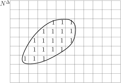
Figure 4 Three scans from viewpoint p₁, p₂, p₃. Set V_i of cell i gives the indices of the viewpoints, whose scans cover cell i. Only one cell (boxed) is covered by all three scans.

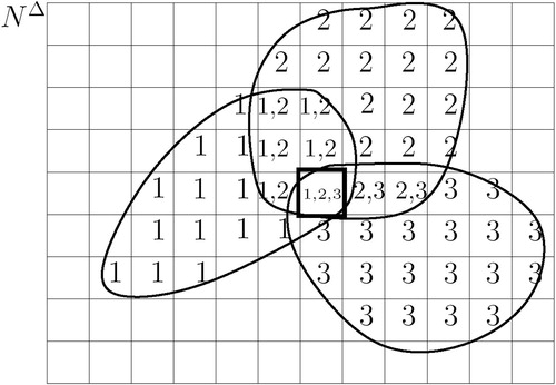
Figure 5 Selected paths from the root to the leaves of a filtered spatial tree (FST).

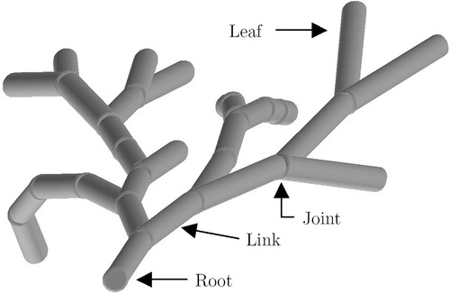
Figure 6 A joint of the FST (frontal view), with u=8, v=1. Each cylinder represents a link in one of 9 (uv+1) joint positions. Note that the center link corresponds to a straight joint position, with a 0° angle between two adjacent links.

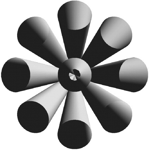
Figure 7 A joint of the FST, with u=4, v=3. Only the centerlines of the links, lying on the surface of concentric cones, are depicted. [Color version available online]

Figure 8 Empirical complexity of a catheter inserted into a brain artery. A fourth-order polynomial was fitted to the observed data from the FST algorithm. A linear fit was found for the data from the ∼FST algorithm. [Color version available online]

Figure 9 The handling of an endoscope can be parameterized using four parameters: l, α, β and d.

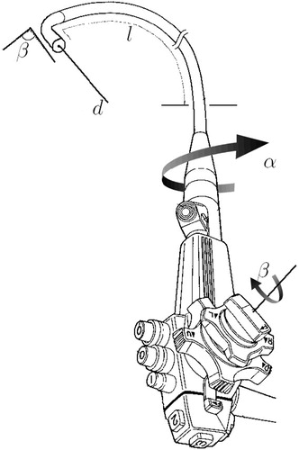
Figure 10 Landmark-based registration. The insertion depth to the biopsy site can be given as an offset to the insertion depth to the main carina.

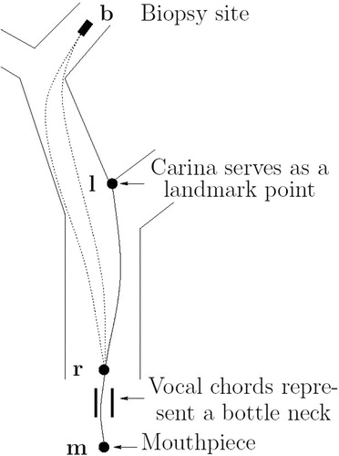
Figure 11 Passive controls for monitoring the endoscope configuration.

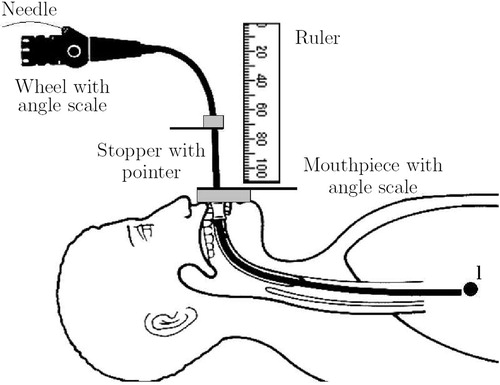
Figure 12 The TBNA protocol, including patient-non-specific instructions and patient-specific parameters (l, α_i, β_i, d_i).

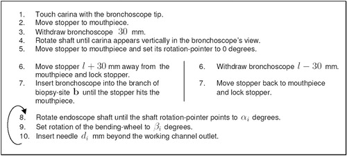
Figure 13 Experimental setup. Olympus GIF-100 with retro-reflective markers inserted into an “M”-shaped calibration path. The endoscope's shape (centerline) was measured in 3D space, using an optical stereo tracking system.

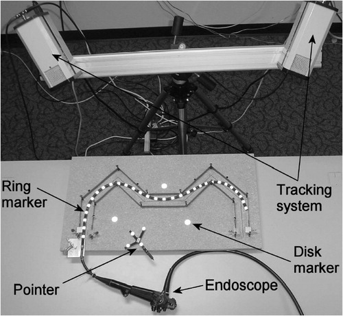
Figure 14 Endoscope model inserted into the calibration path model. Intermediate results (n=44, n′=16, k=2) after the first 13 segments were calculated. All “tentacles” are shown full length. [Color version available online]

Figure 15 Final result (n=44, n′=20, k=4, p=7), showing only the first k=4 links of each tentacle. For the last segment the energy constraint has been relaxed by computing the p=7 smallest energies. The endoscope model largely matches the measured markers of the real endoscope. [Color version available online]

Figure 16 Insertion simulation at 12 different stages: After insertion to a depth of 420 mm, the endoscope became stuck due to insufficient branch diameter. [Color version available online]

Figure 17 Active bending simulation: How far can the Olympus GIF-100 reach into the upper right lobe of the lung phantom? [Color version available online]

Figure 18 The deformation energy decreases from top left to bottom right. [Color version available online]

Figure 19 Experimental setup, showing the lung and head phantom and the endoscope with the biopsy needle.

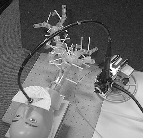
Figure 20 Experimental setup showing the tracking cameras and lung phantom.

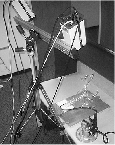
Figure 21 Experimental setup showing the Olympus GIF-100 with reflective markers inserted into the lung phantom.

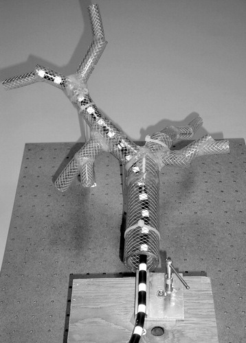
Figure 22 Model accuracy: measured shape. [Color version available online]

Figure 23 Model accuracy: predicted shape. [Color version available online]

Figure 24 Endoscope model (workspace) inserted into a lung model. Target T is represented by an elliptical point cloud. [Color version available online]

Figure 25 The algorithm kCP_Greedy().

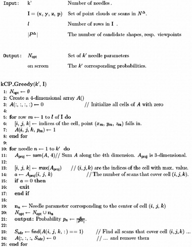
Figure 26 Ten scans of T^Δ, rendered as lit convex hulls of the respective point clouds. [Color version available online]

Figure 27 Same scans as in Figure 26, but each rendered with a 0.5 transparency value (alpha blending). Bending model: f_free. [Color version available online]

Figure 28 Same scans as in Figure 26, but using bending model f_coll. [Color version available online]

Figure 29 Same scans as in Figure 27, but using bending model f_coll. [Color version available online]

Figure 30 Screen shots from the kCP_Greedy() Matlab simulation. Figures (b)–(g) correspond to needles 1–6 in Table I. [Color version available online]

Table I.  Probability of success for each needle placed.

Needle	1	2	3	4	5	6
Probability [%]	42	28	16	4	4	3
Sum	42	71	86	90	94	97