Design, implementation and accuracy of a prototype for medical augmented reality

Figures & data

Figure 1. (a) Typical data displayed during neuronavigation, representing a virtual environment. (b) Three-dimensional geometry data (models) registered and displayed on a live video view. This represents an augmented-reality view. Note the difference between AR and VR. [Color version available online]

Figure 2. Neuronavigators: the precursor of augmented reality. (a) We use the Microscribe as the tool tracker. The position and orientation of the end-effector is shown on the orthogonal slices and 3D model of the phantom skull. After adding a calibrated and registered camera (b), an augmented reality scene can be generated (c). [Color version available online]

Figure 3. Steps required to generate both a neuronavigation system and an augmented reality system. Note that AR represents an extension to neuronavigation and can be performed simultaneously with it. [Color version available online]

Figure 4. The transformations needed to compute the required transformation from the end-effector to the camera coordinates T_EE-C. [Color version available online]

Figure 5. Camera calibration model. Objects in the world coordinate system need to be transformed using two sets of parameters—extrinsic and intrinsic.

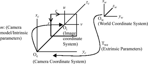
Figure 6. Camera parameter estimation. An initial guess of the extrinsic parameters comes from the DLT method. The observed CCD array points and the corresponding computed values are compared to determine if they are within a certain tolerance. If so, the iteration ends.

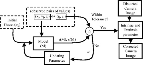
Figure 7. A cube is augmented on the live video from the Microscribe. Three orthogonal views are used to compute the error: (A) represents a close-up view of the pointer (the known location of the cube corner) with the video camera on the x-axis; (B) is the pointer as viewed from the y-axis; and (C) is the pointer viewed from the z-axis. (D) represents an oblique view of the scene with the entire cube viewed. [Color version available online]

Figure 8. Errors of the distorted image. The contours represent error boundaries. Note that for radial distortion at the center (left) there is less than 5 pixels of error and at the corners the errors exceed 25 pixels. The tangential distortion is an order of magnitude less than the radial distortion.

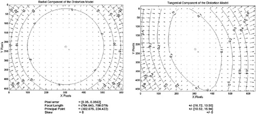
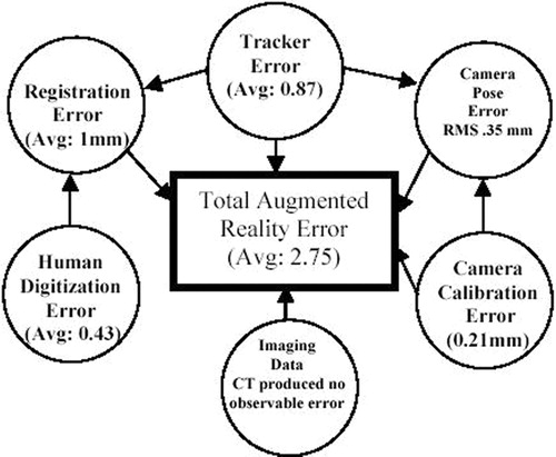
Figure 9. Errors involved in augmented reality.