Figures & data
Figure 1. An image of the planar calibration grid used for estimating the camera parameters. The stereo endoscope was kept static while the calibration object was shown in several arbitrary positions in front of the cameras. [Color version available online]
![Figure 1. An image of the planar calibration grid used for estimating the camera parameters. The stereo endoscope was kept static while the calibration object was shown in several arbitrary positions in front of the cameras. [Color version available online]](/cms/asset/3e1ffc26-ebe8-428e-9a80-85050326144a/icsu_a_123020_f0001_b.jpg)
Figure 2. The epipolar geometry between the stereo cameras reduces the stereo-matching search space to corresponding epipolar lines.
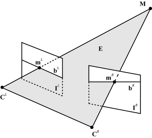
Figure 3. (a) A standard laparoscopic image as viewed by the surgeon. (b) Rectified image as used by the registration algorithm. The warping between introduced and rectified image is visibly small. [Color version available online]
![Figure 3. (a) A standard laparoscopic image as viewed by the surgeon. (b) Rectified image as used by the registration algorithm. The warping between introduced and rectified image is visibly small. [Color version available online]](/cms/asset/181be0f9-85d6-4dcd-9127-4e50d73eede9/icsu_a_123020_f0003_b.jpg)
Figure 4. Several iterations of the registration algorithm showing the evolving PBM lattice and the resulting depth map image. [Color version available online]
![Figure 4. Several iterations of the registration algorithm showing the evolving PBM lattice and the resulting depth map image. [Color version available online]](/cms/asset/e9fbef4d-aea7-4465-ad6f-effea132f03e/icsu_a_123020_f0004_b.jpg)
Figure 5. A schematic illustration of the system for tracking the temporal 3D motion of a surface point by traversing through the temporal and spatial registration transformations St and .
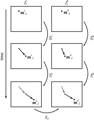
Figure 6. (a and d) Images from the left camera of the stereo rig. (b and e) Two slices from the CT scan at different levels of surface deformation. (c and f) Corresponding 3D plots of the full phantom model surface as reconstructed from the CT data. [Color version available online]
![Figure 6. (a and d) Images from the left camera of the stereo rig. (b and e) Two slices from the CT scan at different levels of surface deformation. (c and f) Corresponding 3D plots of the full phantom model surface as reconstructed from the CT data. [Color version available online]](/cms/asset/b1a98c75-8a81-40db-afbf-1a88b1975cd4/icsu_a_123020_f0006_b.jpg)
Figure 7. The reconstructed 3D surface for four different levels of deformation as captured by 3D CT (a) and the proposed depth recovery method based on combined image rectification and constrained disparity registration (b). [Color version available online]
![Figure 7. The reconstructed 3D surface for four different levels of deformation as captured by 3D CT (a) and the proposed depth recovery method based on combined image rectification and constrained disparity registration (b). [Color version available online]](/cms/asset/432b1550-1332-45c3-aee3-af48ad5af190/icsu_a_123020_f0007_b.jpg)
Figure 8. Scatter plots (a)–(c) illustrate the correlation of the recovered depth change between different levels of deformation by the CT and the proposed technique. [Color version available online]
![Figure 8. Scatter plots (a)–(c) illustrate the correlation of the recovered depth change between different levels of deformation by the CT and the proposed technique. [Color version available online]](/cms/asset/4fa8d163-96e4-4699-ab34-b33574dedb23/icsu_a_123020_f0008_b.jpg)
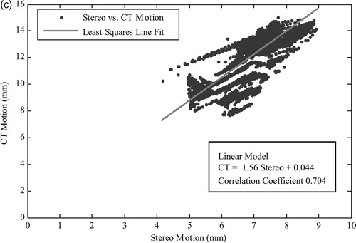
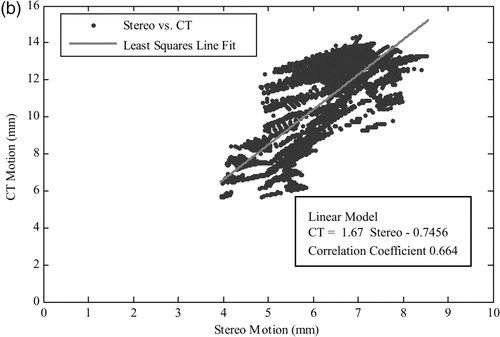
Table I. Evaluation of the regression between the recovered motion and the ground-truth CT motion for the scaled-up phantom constructed for this study.
Figure 9. A pair of stereo-images (a and e) from an in vivo stereoscopic laparoscope sequence and three temporal frames of the reconstructed depth map (b–d) and their corresponding 3D rendering results (f–h). Arrows indicate visible errors in the recovered depth due to specular highlights. [Color version available online]
![Figure 9. A pair of stereo-images (a and e) from an in vivo stereoscopic laparoscope sequence and three temporal frames of the reconstructed depth map (b–d) and their corresponding 3D rendering results (f–h). Arrows indicate visible errors in the recovered depth due to specular highlights. [Color version available online]](/cms/asset/7f9439cf-fa81-4b7f-8534-f80d94861c9f/icsu_a_123020_f0009_b.jpg)
Figure 10. (a) A laparoscopic image where specular highlights have been detected through thresholding. (b) Corresponding PBM lattice where control points affected by a large specular highlight have been highlighted. (c) The 3D rendering result of the reconstruction after interpolating across erroneous control points. [Color version available online]
![Figure 10. (a) A laparoscopic image where specular highlights have been detected through thresholding. (b) Corresponding PBM lattice where control points affected by a large specular highlight have been highlighted. (c) The 3D rendering result of the reconstruction after interpolating across erroneous control points. [Color version available online]](/cms/asset/ac27aedf-3ed6-467f-bf55-43b9a9139df0/icsu_a_123020_f0010_b.jpg)