Figures & data
Figure 2. X-ray showing the final position of the implant Citation[10].
![Figure 2. X-ray showing the final position of the implant Citation[10].](/cms/asset/de6df08b-3887-4de4-b289-b4fe6c9d25fa/icsu_a_143200_f0002_b.gif)
Figure 4. The implant aligned along the trochlear groove. The plane contains both the centerline of the implant and the trochlear groove of the knee model. Small dots represent each point of the knee collected by the CT imagery. [Color version available online]
![Figure 4. The implant aligned along the trochlear groove. The plane contains both the centerline of the implant and the trochlear groove of the knee model. Small dots represent each point of the knee collected by the CT imagery. [Color version available online]](/cms/asset/b8a7fed3-50d7-4246-b3cc-18f488777d4b/icsu_a_143200_f0004_b.gif)
Figure 5. Implant in four positions rotated in 15° increments about the distal tip. [Color version available online]
![Figure 5. Implant in four positions rotated in 15° increments about the distal tip. [Color version available online]](/cms/asset/2fb42952-33f1-48e5-a965-b4b74961c620/icsu_a_143200_f0005_b.gif)
Figure 7. Cellular decomposition: the resulting cells, marked by circular icons, are shown in step d.
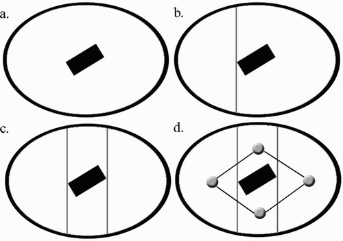
Figure 10. The circular cutting tool tip leaves ridges known as scallops. Scallop height is dependent on the amount of overlap of the cuts made by the tool.
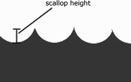
Figure 11. Step 1: Find the intersection of the start plane and knee model. Circles represent discrete points a set distance apart on the resulting intersection. Note that points on the intersection that fall outside the implant area are not shown.
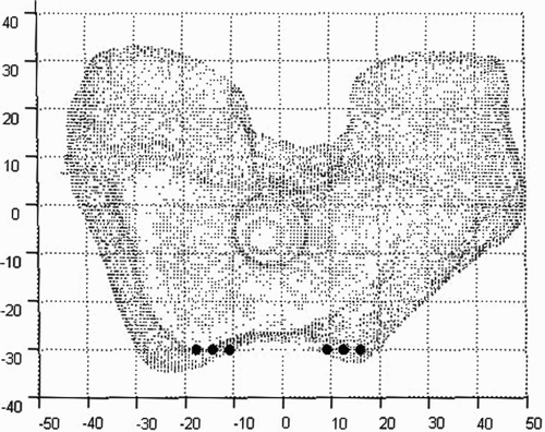
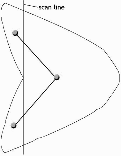
Figure 13. Pruning sweep lines for step 4 and identifying critical points for step 5. [Color version available online]
![Figure 13. Pruning sweep lines for step 4 and identifying critical points for step 5. [Color version available online]](/cms/asset/e34249b1-f597-4d7d-9500-8ac6b6d2ea6b/icsu_a_143200_f0013_b.gif)
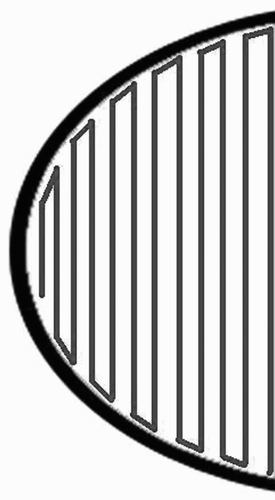
Figure 14. Step 5: Fix sweep lines that cross the negative area of the implant. Connect the two cells (as indicated by the arrow) for a single trajectory that covers the entire area to be milled. [Color version available online]
![Figure 14. Step 5: Fix sweep lines that cross the negative area of the implant. Connect the two cells (as indicated by the arrow) for a single trajectory that covers the entire area to be milled. [Color version available online]](/cms/asset/00cd77b7-0538-451a-889f-bc0533873e0f/icsu_a_143200_f0014_b.gif)
Figure 16. Typical trajectory as formed by virtual forces. The first position demonstrates the surface as a repulsive force, the second demonstrates it as an attractive force. [Color version available online]
![Figure 16. Typical trajectory as formed by virtual forces. The first position demonstrates the surface as a repulsive force, the second demonstrates it as an attractive force. [Color version available online]](/cms/asset/9c1393b8-7abf-481d-bd75-b94b9b2d3e5e/icsu_a_143200_f0016_b.gif)
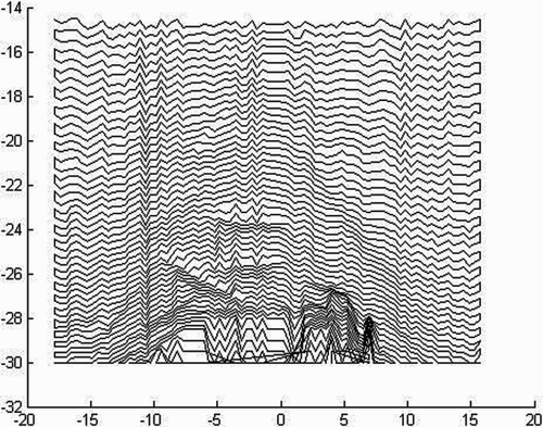
Figure 17. Simulated paths across a fourth-order polynomial. Curves further away from the surface correspond to smaller values of Kg. The polynomial was chosen using least squares to best fit the surface model points. [Color version available online]
![Figure 17. Simulated paths across a fourth-order polynomial. Curves further away from the surface correspond to smaller values of Kg. The polynomial was chosen using least squares to best fit the surface model points. [Color version available online]](/cms/asset/763453ea-3039-4862-8635-879ad2c1e5d0/icsu_a_143200_f0017_b.gif)
![Figure 1. CAD drawing of MBARS. [Color version available online]](/cms/asset/764aec2c-f11f-4abe-9104-8b04dc1f9826/icsu_a_143200_f0001_b.gif)
![Figure 3. Two views of the trochlear component surface model. [Color version available online]](/cms/asset/ee95f382-4b08-451d-98b9-b7b8775bd2a2/icsu_a_143200_f0003_b.gif)
![Figure 6. Implant fitted on patellofemoral surface. [Color version available online]](/cms/asset/c4e81ff5-aaea-4936-8f4b-887b07c6712e/icsu_a_143200_f0006_b.gif)
![Figure 15. Mapping from R2 to U. [Color version available online]](/cms/asset/3d14d0ef-0d68-4e7d-bee9-25f9105fe0a9/icsu_a_143200_f0015_b.gif)