Figures & data
Figure 1. (a) The color-coded instrument. (b) The averaged color distribution in the H-S plane for 3000 laparoscopic images, together with the H-S occupation of the colored band in the highlighted oval. (c) The segmented image with superimposed geometric features needed for localization. [Color version available online.]
![Figure 1. (a) The color-coded instrument. (b) The averaged color distribution in the H-S plane for 3000 laparoscopic images, together with the H-S occupation of the colored band in the highlighted oval. (c) The segmented image with superimposed geometric features needed for localization. [Color version available online.]](/cms/asset/e33269f3-b760-49cd-8698-869828c36bd9/icsu_a_220998_f0001_b.gif)
Figure 2. Schematic representation of the image processing steps needed for color segmentation: the pre-processing phase is shown at the top, while the lower part shows the intra-operative segmentation process applied to two endoscope images. See text for a detailed description. [Color version available online.]
![Figure 2. Schematic representation of the image processing steps needed for color segmentation: the pre-processing phase is shown at the top, while the lower part shows the intra-operative segmentation process applied to two endoscope images. See text for a detailed description. [Color version available online.]](/cms/asset/0d126ee5-eea0-44aa-891f-27e713de2624/icsu_a_220998_f0002_b.gif)
Figure 3. (a) Angles defining local orientation of an object. (b) Pinhole camera model.
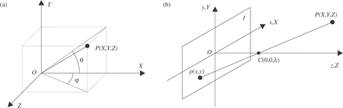
Figure 4. Line convergence due to perspective transform. (a) and (b) are images of the instrument placed at different angles with respect to the image plane. The highlighted lines in (a) and (b) correspond to the first two global maxima of the Hough transform of the images (c).
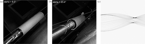
Figure 5. Experimental setup for measuring distances and angles.
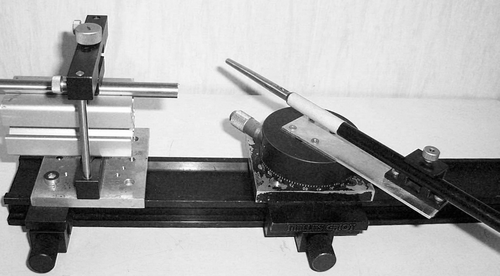
Figure 6. Experimental relation φ = φ(α, θ).
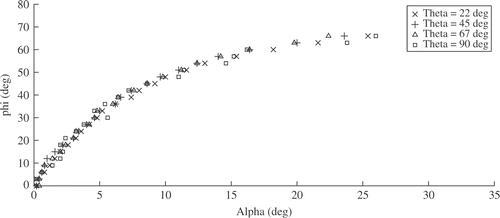
Figure 7. Experimental relation φ = φ(α, Z).
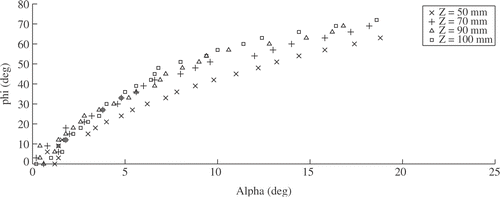
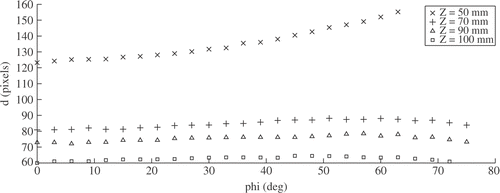
Figure 8. Experimental relation d = d(φ, Z).