New approaches to online estimation of electromagnetic tracking errors for laparoscopic ultrasonography

Figures & data

Figure 1. Coordinate frames associated with our hybrid magneto-optic tracking setup to localize the laparoscope and the tip of the laparoscopic ultrasound.

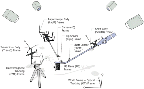
Figure 2. Screenshot of axis segmentation. Lines classified as belonging to the transducer tip edges are automatically colored yellow; lines belonging to the transducer (but not to the edges) are colored blue; and the corrected transducer axis is the thick red line. Lines belonging to the pencil are rejected (colored green), because they do not match the measured transducer axis rotation. [Color version available online.]

Figure 3. Back-projection of a segmented line and its comparison to the transducer tip axis measured by EMT. [Color version available online.]

Figure 4. Back-projection of four segmented lines, which generates four planes and their corresponding normals n₁, n₂, n₃, and n₄ (plane coloring according to Figure 2). For each plane j, its distance d_j to b_C and angle α_j to d_C are computed. We suppose that all four planes satisfy |α_j| < 5° and |d_j| < 30 mm. Because d₁ is the maximum positive distance from b_C, and d₄ the maximum negative distance from b_C, we can set d_posmax = d₁ and d_negmax = d₄. If |d_posmax − d_negmax| = |d₁ − d₄| stays within 10 ± 2 mm, we continue our computations. For all distances i unequal d_posmax and d_negmax, we check whether d_posmax − d_i < 2 mm or d_i − d_negmax < 2 mm. All planes not satisfying this criterion are excluded from further computations, as for plane 2 (blue). Using the remaining three yellow planes, a mean plane (red) defined by and is determined. The transducer tip axis can finally be translated along for d_est = 0.5(d₁ + d₄) mm and rotated by around . [Color version available online.]

Figure 5. Setup for error evaluation.

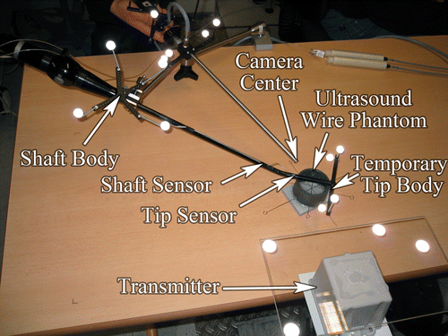
Figure 6. ROC curves for error prediction. (a) Prediction of an error of 5.0 mm or greater. (b) Prediction of an error of 7.5 mm or greater.

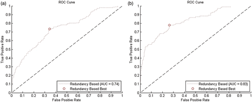
Table I.  Distortion detection rate by our distrust level without distortion, with static, and with dynamic field distortion.

Distortion		True	False
Without	positive	40.0%	10.0%
	negative	30.0%	20.0%
Static	positive	100.0%	0.0%
	negative	0.0%	0.0%
Dynamic	positive	73.8%	13.8%
	negative	12.4%	0.0%
Average	positive	71.3%	7.9%
	negative	14.1%	6.7%

Table II.  Receiver operating characteristic key figures for prediction of distortion errors of at least 2.5, 5, 7.5, and 10 mm.

	AUC	Jmax	δthresh	TPR	SPC	FPmin	FNmax
2.5 mm	0.65	0.24	6.26	0.91	0.33	0.84	6.44
5.0 mm	0.74	0.39	11.34	0.74	0.66	0.84	13.69
7.5 mm	0.83	0.52	13.98	0.78	0.74	0.85	13.69
10.0 mm	0.86	0.67	27.75	0.72	0.94	0.88	14.29

Table III.  Overlay errors in an undistorted and a distorted field.

	Min	Mean	SD	RMS	Max
Undistorted (mm)
Projected OT	0.11	2.67	1.38	3.00	7.57
Projected EMT	0.17	3.57	2.49	4.35	11.81
Redundancy-based correction	0.38	3.73	1.99	4.23	11.19
Vision-based correction	0.20	2.91	1.75	3.39	9.51
Distorted (mm)
Projected OT	0.05	1.81	1.02	2.08	6.10
Projected EMT	0.11	10.03	7.81	12.71	39.84
Redundancy-based correction	0.07	8.55	7.63	11.45	36.66
Vision-based correction	0.17	7.77	6.60	10.19	38.43

Figure 7. Ultrasound plane augmented on the laparoscope video – the red line is added manually to show the extension of the straight wire, which matches its ultrasound image. [Color version available online.]