Double-bundle ACL reconstruction: Novice surgeons utilizing computer-assisted navigation versus experienced surgeons

Figures & data

Figure 1. Mean preoperative tibial ACL footprint as determined using sagittal and coronal MRI with overlay on an axial image. The maximum sagittal and coronal widths of the tibia were determined, and the anterior, posterior, medial and lateral extents of the ACL were measured on MRI and expressed as a percentage of the maximum tibial width from the most anterior and medial aspects of that width. The mean center of the footprint is also expressed as a percentage width.

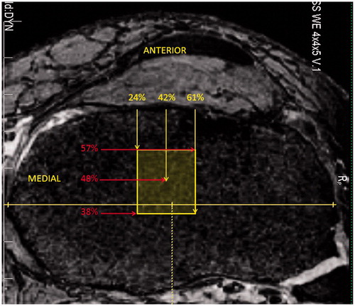
Figure 2. Computer-assisted navigation graphical user interface as used by the novice surgeon group, allowing the operator to understand the location on the tibial plateau and lateral femoral condyle of the right knee. (A) The interface for the tibial side. (B) The interface for the femoral side.

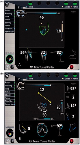
Figure 3. Tibial measurements were made using sagittal and coronal MR images. The maximum sagittal width of the tibia parallel to the joint line, S, was measured and copied to all images (A). The slice at which the AM or PL tunnel broke the subchondral bone of the tibial plateau was located and measured perpendicular to line S. The distance S¹ was expressed as a percentage of the maximum sagittal width (B). The maximum coronal width was measured and represented by line C (C). The slice at which the AM or PL tunnel broke the subchondral bone was identified and measured perpendicular to line C. The distance C¹ was expressed as a percentage of the maximum coronal width (D).

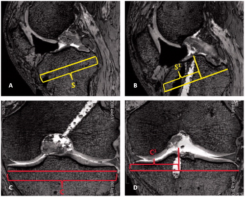
Figure 4. Femoral measurements were made on sagittal MR images of the lateral femoral condyle using modifications to the quadrant technique described by Bernard et al. [4]. First, the most proximal aspect of the femoral notch was identified, correlating to Blumensaat’s line (A). Next, the maximum sagittal width along Blumensaat’s line (W) was identified, measured, and copied to all images (B). The most distal aspect of the lateral femoral condyle was then identified and a line drawn tangential to that point. The perpendicular distance from Blumensaat’s line to this line was the notch height, H (C). Lastly, the slice at which the AM or PL tunnel broke the subchondral bone of the lateral femoral condyle was identified. Measurements were made perpendicular to lines W and H in order to locate the center of the tunnel. The center of the tunnel was expressed as a percentage along Blumensaat’s line and the notch height, displayed as W¹ and H¹, respectively (D).

Table I.  Preoperative dimensions of the tibial ACL footprint.

	Distance (mm)	Percentage depth
Sagittal measurements
Tibial depth (A-P)	57 ± 5.0	NA
Anterior footprint	14 ± 2.9	24 ± 4.5
Center of footprint	24 ± 2.6	42 ± 3.7
Posterior footprint	35 ± 2.7	61 ± 4.3
Footprint width	21 ± 2.0	37 ± 4.7
Coronal measurements
Tibial width (M-L)	77 ± 5.6	NA
Medial footprint	30 ± 3.7	39 ± 2.8
Center of footprint	37 ± 3.5	48 ± 2.1
Lateral footprint	44 ± 3.5	57 ± 2.1
Footprint width	14 ± 1.5	18 ± 2.4

Table II.  Comparison of tunnel placement by experienced and novice surgeons expressed as percentage values.

	Femur				Tibia
	Blumensaat’s		Notch height		Sagittal		Coronal
	AM	PL	AM	PL	AM	PL	AM	PL
Experienced	30 ± 7.2	37 ± 7.2	5.9 ± 6.5	42 ± 14	37 ± 7.4	53 ± 8.7	43 ± 1.8	49 ± 2.2
Novice	43 ± 10	46 ± 7.3	11 ± 11	49 ± 12	32 ± 7.1	54 ± 5.8	43 ± 3.3	47 ± 3.0
p-value	0.0073*	0.0098*	0.22	0.29	0.18	0.75	0.96	0.10

*statistically significant.

Figure 5. Centers of the anteromedial (AM) and posterolateral (PL) tunnels mapped on the lateral femoral condyle for each knee studied. Tunnel location was determined using the extension of Blumensaat’s line and notch height on sagittal MRI. Novice surgeon computer aided AM and PL tunnels were significantly anterior to tunnels made by experienced surgeons. The range of AM and PL centers from previous anatomic studies are also mapped on the lateral femoral condyle for comparison.

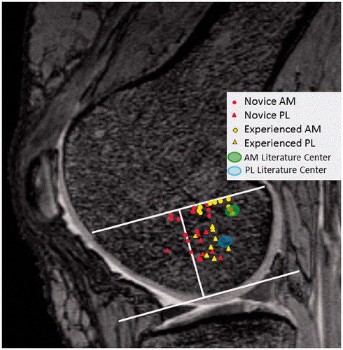
Table III.  Overview of studies evaluating the femoral and tibial insertion of the AM and PL bundles compared to tunnel position in the present study. All numerical values are percentages.

		Femur				Tibia
		Blumensaat’s		Notch height		Sagittal		Coronal
Author	Study type	AM	PL	AM	PL	AM	PL	AM	PL
Colombet et al. [5]	Radiologic (XR)	26.4	32.3	25.3	47.6	36.0	52.0
Lorenz et al. [11]	Radiologic (CT)	21.0	27.0	22.0	45.0	41.0	52.0	52.0*	50.0*
Pietrini et al. [12]	Radiologic (XR)	21.6	28.9	14.2	42.3	36.3	51.0	44.2	50.1
Tsukada et al. [17]	Anatomic	25.9	34.8	17.8	42.1	37.6	50.1	46.5	51.2
Yamamoto et al. [26]	Radiologic (XR)	25.0	29.0	16.0	42.0
Zantop et al. [28]	Radiologic (XR)	18.5	29.3	22.3	53.6	30.0	44.0
Anthony et al.	Experienced	30 ± 7.2	37 ± 7.2	5.9 ± 6.5	42 ± 14	37 ± 7.4	53 ± 8.7	43 ± 1.8	49 ± 2.2
	Novice	43 ± 10	46 ± 7.3	11 ± 11	49 ± 12	32 ± 7.1	54 ± 5.8	43 ± 3.3	47 ± 3.0

*Lorenz et al. made tibial plateau coronal references from the lateral border of the tibial plateau, compared with the tibial plateau coronal references made from the medial border in the present study and in those by other groups [20, 31].

Bernard M, Hertel P, Hornung H, Cierpinski T. 1997. Femoral insertion of the ACL. Radiographic quadrant method. Am J Knee Surg 10(1):14–21; discussion 21–22

 PubMedGoogle Scholar

Colombet P, Robinson J, Christel P, et al. 2006. Morphology of anterior cruciate ligament attachments for anatomic reconstruction: A cadaveric dissection and radiographic study. Arthroscopy 22(9):984–92

 PubMed Web of Science ®Google Scholar

Lorenz S, Elser F, Mitterer M, et al. 2009. Radiologic evaluation of the insertion sites of the 2 functional bundles of the anterior cruciate ligament using 3-dimensional computed tomography. Am J Sports Med 37:2368–76

 PubMed Web of Science ®Google Scholar

Pietrini SD, Ziegler CG, Anderson CJ, et al. 2011. Radiographic landmarks for tunnel positioning in double-bundle ACL reconstructions. Knee Surg Sports Traumatol Arthrosc 19(5):792–800

 PubMed Web of Science ®Google Scholar

Tsukada H, Ishibashi Y, Tsuda E, et al. 2008. Anatomical analysis of the anterior cruciate ligament femoral and tibial footprints. J Orthop Sci 13:122–9

 PubMed Web of Science ®Google Scholar

Yamamoto Y, Hsu WH, Woo SL, et al. 2004. Knee stability and graft function after anterior cruciate ligament reconstruction: A comparison of a lateral and anatomical femoral tunnel placement. Am J Sports Med 32:1825–32

 PubMed Web of Science ®Google Scholar

Zantop T, Wellmann M, Fu FH, Petersen W. 2008. Tunnel positioning of anteromedial and posterolateral bundles in anatomic anterior cruciate ligament reconstruction: Anatomic and radiographic findings. Am J Sports Med 36:65–72

 PubMed Web of Science ®Google Scholar

Abebe ES, Utturkar GM, Taylor DC, et al. 2011. The effects of femoral graft placement on in vivo knee kinematics after anterior cruciate ligament reconstruction. J Biomech 44(5):924–9

 PubMed Web of Science ®Google Scholar

Klos T, Habets R, Banks AZ, et al. 1998. Computer assistance in arthroscopic anterior cruciate ligament reconstruction. Clin Orthop Relat Res 354:65–9

 PubMedGoogle Scholar