New method to estimate the possibility of natural pregnancy using computer-assisted sperm analysis

Figures & data

Figure 1.  Examples of the actual distribution and theoretical distribution of sperm energy. X and Y are Isobe plot variables defined from the new sperm energy theory scatter diagrams of an actual sperm distribution are compared to the theoretical distribution calculated based on the new sperm energy theory. The slope of the regression line in the Isobe plot equals the Isobe coefficient (K value). The actual and theoretical distribution curves are respectively plotted with the actual ratio of the existing sperm number, or the theoretical existing probability density (= P) on the vertical axis, and with the square of the amplitude of lateral head displacement (ALH) (=t) on the horizontal axis. A theoretical distribution chart was obtained using the Isobe coefficient. The correctness of the hypothesis (new sperm energy theory) is demonstrated by the perfect agreement between the actual and theoretical distributions.

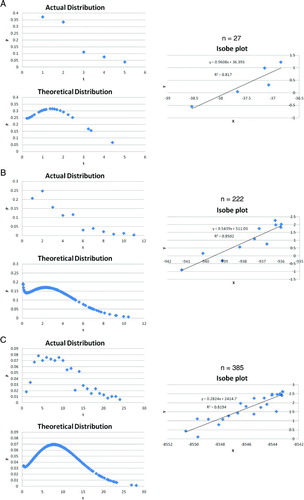
Figure 2.  Relationship between sperm concentration/percent motility and the sperm energy index calculated based on the new sperm energy theory. The mechanical energy of a single sperm can be expressed as K × the square of the amplitude of lateral head displacement (ALH). SEI and MEI are defined as below. SEI indicates the total mechanical energy of the sperm existing in a visual field of a CASA measurement, and MEI indicates the mean mechanical energy of one sperm existing in a measurement field: SEI = nKλ/100; MEI = Kλ. Where, λ is the mean value of the square of measured ALH obtained for the total sperm count in a single measurement field, and n is the number of measured motile sperm that could be traced completely from the start to end of the measurements in a single visual field. The Isobe coefficient (K value) is obtained as the slope of the regression line (Eq.(2.9)) of an Isobe plot scatter diagram based on the new sperm energy theory using the least squares method. SEI was positively correlated with both sperm concentration and percent motility.

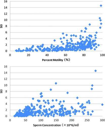
Figure 3.  Sperm energy index in the control and sterile groups. A scatter diagram with MEI plotted on the vertical axis and SEI on the horizontal axis in the sterile and control groups. All subjects with (MEI)/(SEI) > 2 were in the sterile group. The MEI-SEI ratio is in inverse proportion to motile sperm concentration. The ratio of subjects who fulfilled the criteria of (MEI)/(SEI) > 2 against the total number of subjects in the sterile group was 43.4% (56/129). The MEI-SEI ratio can be criteria for estimating necessity of treatment.

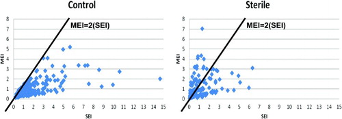
Figure 4.  Variability in the sperm energy index on different days and times from the same subjects. Scatter diagrams plotted with SEI/MEI data of semen samples collected on different days and times from two representative subjects each from the control and sterile groups. The findings showed that (MEI)/(SEI) >2 was not seen in either of the two representative cases (control cases 1 and 2) from the control group. Some samples obtained from two representative cases (sterile cases 1 and 2) in the sterile group fulfilled the criteria of (MEI)/(SEI) > 2.

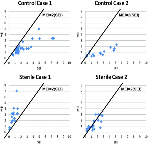
Figure 5.  Percent motility and sperm concentration in the control and sterile groups. A scatter diagram with percent motility plotted on the vertical axis and sperm concentration on the horizontal axis. The top pane is a plot of the control group, and the bottom pane is a plot of the sterile group. None of the subjects produced natural pregnancy when sperm concentration was less than 35 × 10⁶/ml. The ratio of subjects with sperm concentrations < 20 × 10⁶ /ml against the total number of subjects in the sterile group was 3.9% (5/129). The ratio of subjects with percent motility > 50% in the fertile group against the total number of subjects in both the fertile and sterile groups was 58.29% (109/187). The ratio of subjects with sperm concentration > 20 × 10⁶ /ml in the fertile group against the total number of subjects in both the fertile and sterile groups was 50.99% (129/253).

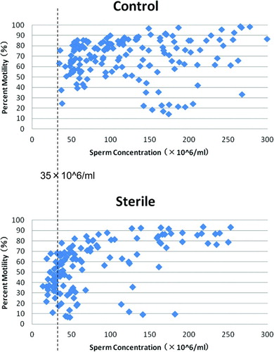
Table 1. Relationship between the SEI and the probability of predicting fertile subjects.

SEI	The number of subjects in fertile group	The number of subjects in sterile group	Percent of fertile subjects
>7	8	0	100
>6	9	1	90
>5	13	3	81.25
>4	22	6	78.57
>3	37	9	80.43
>2	61	23	72.62
>1	106	51	67.52
>0.9	110	56	66.27
>0.8	110	59	65.09
>0.7	117	68	63.24
>0.6	118	73	61.78
>0.5	123	82	60
>0.4	125	89	58.41
>0.3	125	92	57.6
>0.2	128	102	55.65
>0.1	129	113	53.31
>0.05	129	123	51.19
>0	129	129	50

In total, 129 subjects were selected from the control group and classified as the fertile group in order of the sample measurement date. The larger the SEI, the higher was the likelihood of predicting fertile subjects. The probability of predicting fertile subjects was approximately 60% with a SEI of > 0.5, 70% with a SEI of > 1, 80% with a SEI of > 3, and 90% with a SEI of > 6. SEI can be an index of anticipating natural pregnancy in cases where (MEI)/(SEI) is < 2.