
Figures & data
Figure 1. (A) CVs of 1 mmol L–1 Fe(CN)63–/4– on the various NiONPs–CPEs with the mass ratios of NiONPs to graphite powder were 1:2 (a), 1:3 (b), 1:4 (c), and 1:5 (d) (Scan rate: 50 mV s–1), (B) the plot of the peak current vs. H2O2 concentration for the various NiONPs‐CPEs in 0.1 M PBS (pH 7.0) at 0.4 V vs. Ag/AgCl.
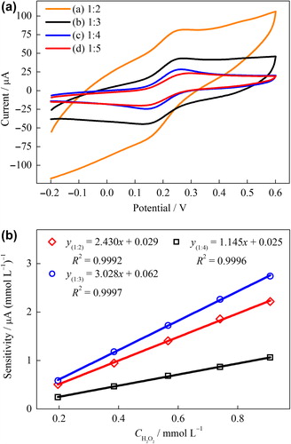
Table I. Comparisons of electrochemical characteristics of the NiONPs–CPEs were prepared at the various mass ratio of NiONPs/graphite toward the redox probe of Fe(CN)63–/4– (scan rate = 50 mVs–1).
Figure 2. (A) CVs of the UCPE (a) and NiONPs–CPE (b) at scan rate 10 mVs–1, (B) the plot of the peak current vs. the square root of the scan rate for NiONPs‐CPE (inset: CVs at different scan rates) in 0.1 mol L–1 KCl solution containing 1 mmol L–1 Fe(CN)63–/4–.
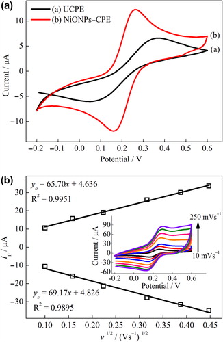
Figure 3. The Nyquist curves of the (a) UCPE and (b) NiONPs–CPE in 0.1 mmol L–1 KCl solution containing 1 mmolL−1 Fe(CN)63–/4–.
Figure 4. (A) CVs of the UCPE and NiONPs–CPE in the absence and presence of 1 mmol L–1 H2O2 (scan rate = 50 mVs–1) in 0.1 mmol L–1 PBS (pH 7.0). (B) Amperometric responses of the UCPE and NiONPs–CPE for the oxidation of H2O2 in 0.1 M PBS (pH 7.0) at 0.4 V vs. Ag/AgCl.
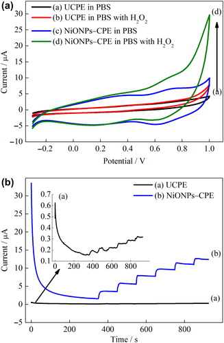
Figure 5. The effect of working potential on the amperometric response of H2O2 in 0.1 mmol L−1 PBS (pH 7.0).
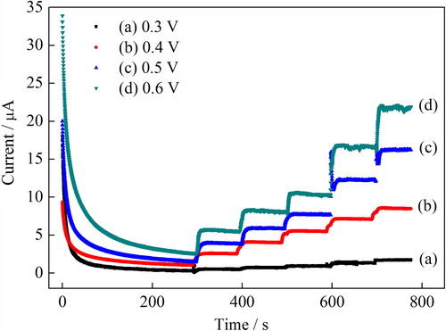
Figure 6. The sensitivity of the GOD–NiONPs–CPE as a function of buffer pH in 0.1 mmol L–1 PBS at 0.4 V vs. Ag/AgCl.
Figure 7. (A) Calibration curve of the GOD–NiONPs–CPE for glucose in 0.1 M PBS (pH 7.0) at 0.4 V vs. Ag/AgCl. (inset: linear working ranges plots), (B) Substrate concentration/current response vs. substrate concentration plot (Hanes–Woolf plot).
Figure 8. Amperometric responses of the glucose biosensor upon addition of AA (0.1 mmol L–1, DA (0.1 mmol L–1), and UA (0.1 mmol L–1) in 0.1 M PBS (pH 7.0) at 0.4 V vs. Ag/AgCl.
Table II. Effects of interferences on glucose response.
Table III. The determination of glucose levels in human serum samples.