Acyclovir-loaded sorbitan esters-based organogel: development and rheological characterization

Figures & data

Table 1. Composition of various formulations.

Smix ratio (Kw)	Different components in formulations (%w/w)
	Formulation code	ACV	IPM	Smix	DDW
1:1 (Figure 1A)	NEOG A	0.05	61.30	33.00	5.65
1:2 (Figure 1B)	NEOG B	0.05	55.60	37.00	7.43
1:3 (Figure 1C)	NEOG C	0.05	48.00	32.00	19.95

NEOG_A–C: nanoemulsion organogel formulations; ACV: acyclovir; IPM: isopropyl myristate; Smix: surfactant mixture; DDW: double-distilled water.

Figure 1. Pseudo-ternary phase diagrams indicating w/o nanoemulsion and organogel region at diffierent Smix ratios (A) K_w = 1:1, (B) K_w =1:2 and (C) K_w = 1:3, where K_w=Smix ratio (Span 60/Tween 80).

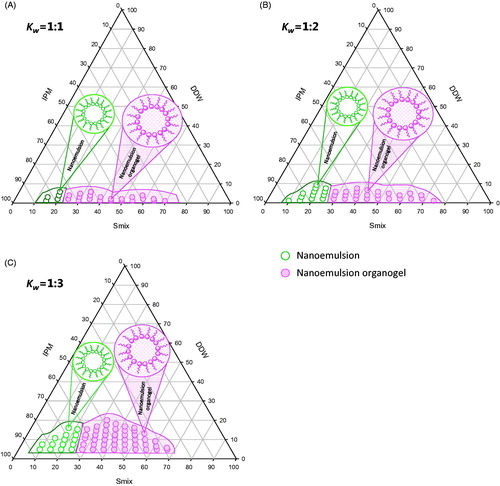
Figure 2. Graph showing variation in turbidity and viscosity as a function of DDW for w/o nanoemulsion at difierent Smix ratios (A) K_w = 1:1, (B) K_w =1:2 and (C) K_w = 1:3, where, K_w=Smix ratio (Span 60/Tween 80).

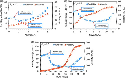
Figure 3. Temperature dependent loss of elastic modulus, G′ (circles), and viscous modulus, G″ (diamonds), and a curve between Tan δ versus Temperature (triangles), with minima at Tg of (A) NEOG A, (B) NEOG B and (C) NEOG C. The curves are plotted by the best sigmoidal fit of the data points.

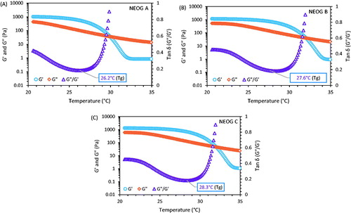
Figure 4. Frequency (ω) dependence of G′ (circles) and G″ (diamonds) in three organogel systems (A) NEOG A, (B) NEOG B and (C) NEOG C. Relaxation exponents were calculated from their slopes.

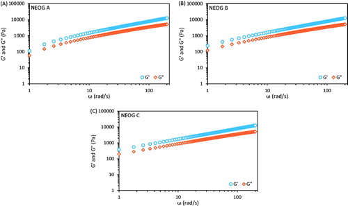
Table 2. Rheological characterization of ACV-loaded NEOG formulations.

		Relaxation exponent and fractal dimension of NEOG
		G′		G″
Formulation code	Transition temperature (Tg) in °C	Relaxation exponent (Δ′)	Fractal dimension (Df)	Relaxation exponent (Δ″)	Fractal dimension (Df)
NEOG A	26.2	0.705	1.732	0.632	1.833
NEOG B	27.6	0.684	1.762	0.611	1.861
NEOG C	28.3	0.661	1.793	0.588	1.890

NEOG_A–C: nanoemulsion organogel formulations.

G′ and G″ represent elastic and viscous modulus, respectively.

Figure 5. Percent drug released versus time curve. The inset shows log (% drug released) versus log T to obtain a power law exponent, which correlates well with direct fitting of the curve to the power law equation.

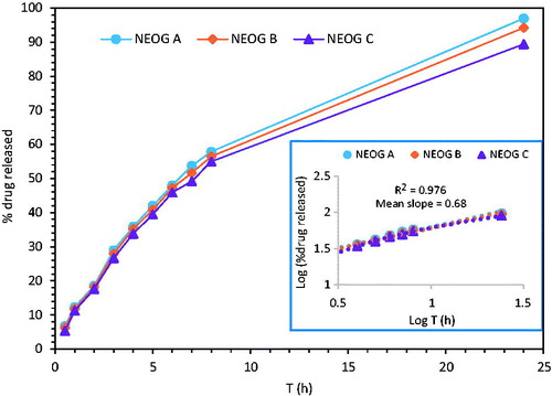
Table 3. In vitro release rate and skin permeation of ACV from various NEOG formulations.

		Skin permeation
Formulation code	Release rate (%/h^0.7/cm^2)	Lag time, L (min)	Flux, J (μg/h/cm^2)	Permeability coefficient, P (cm^2/h)	Diffusion coefficient, D (cm^2/h)
NEOG A	11.04	20	6.91	7.1 × 10^−2	10.5 × 10^−4
NEOG B	10.72	25	6.66	7.0 × 10^−2	8.5 × 10^−4
NEOG C	10.18	30	6.34	6.9 × 10^−2	7.1 × 10^−4

NEOG_A–C: nanoemulsion organogel formulations.

Figure 6. Cumulative drug permeated through hairless pig skin versus time curve.

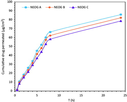
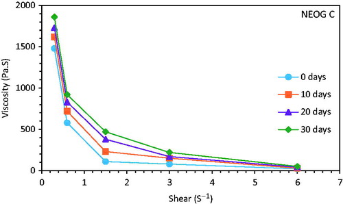
Figure 7. A typical flow curve in between viscosity versus shear of ACV-loaded NEOG C formulation at 0 days (circle), 10 days (squares), 20 days (triangles) and 30 days (diamonds).