Letters to the Editor

Figures & data

Figure 1. (a) Base case and (b) baseline modeled one hour ozone change vs. resulting ozone concentration, August 15-September 14, 2006.

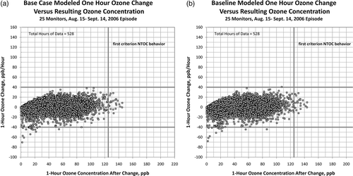
Figure 2. Modeled and observed ozone at Wallisville, August 16, 2006.

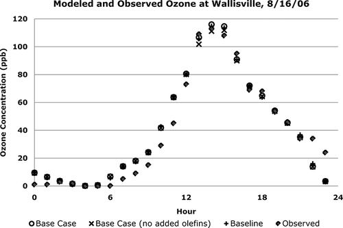
Figure C1. Observed 1-hr and maximum 8-hr (line) ozone concentrations measured at three monitors on September 7, 2006. Arrows indicate 1-hr resultant wind vectors. The lower right is a map of Houston with the locations of the monitors.

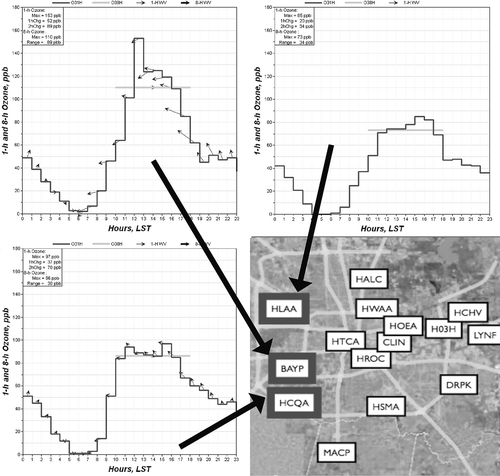
Figure C2. (a) Observed and (b) modeled 1-hr and maximum 8-hr (line) ozone at Bayland Park (BAYP) monitor for September 7, 2006. Small hourly arrows are resultant wind observed and modeled at site each hour.

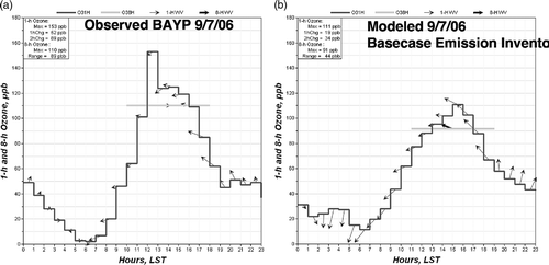
Figure C3. Ozone time series measured at the (a) Deer Park (DRPK) monitor and (b) predicted by the regulatory air quality model using the base case emission inventory. Arrows indicate 1-hr resultant wind vectors, the straight line the 8-hr maximum ozone concentrations.

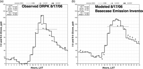
Figure C4. Plot (a) shows for the base case emission inventory, the 1-hr ozone predicted cell-by-cell for 1400 -1500 LST on August 17, 2006. The small diamonds mark monitor sites, but their shading represents observed ozone for the same time and on the same scale. The region shown in black is predicted to be above 120 ppb. Plot (b) shows the observed and predicted 1-hr ozone at each monitor site within the black area of (a). Only two close together monitors reported ozone [H11022]120 ppb, but the model predicted that all monitors over the large region, including those below 85 ppb, were experiencing close to 140 ppb of 1-hr ozone. This model prediction fails the criteria of “spatially-limited, high ozone” associated with monitor-based NTOC phenomena described in our paper.