811
Views
7
CrossRef citations to date
0
Altmetric
Technical Papers

Improvements to Standard Methodologies for the Analytical Determination of Metals in Stationary-Source Emissions Samples

, , &
Pages 764-770 | Published online: 10 Oct 2011

Figures & data

Figure 1. The calibration relationship obtained for Mn in a stationary-source sample matrix showing a fit to a second-order polynomial (solid line; squared correlation coefficient r2 = 0.9997) and a first-order polynomial relationship (dotted line; r2 = 0.991). The calibration points are shown with their uncertainties at the 95% confidence level in the x- and y-axes.
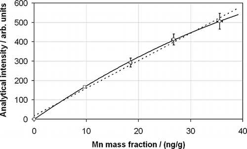
Figure 1. The calibration relationship obtained for Mn in a stationary-source sample matrix showing a fit to a second-order polynomial (solid line; squared correlation coefficient r2 = 0.9997) and a first-order polynomial relationship (dotted line; r2 = 0.991). The calibration points are shown with their uncertainties at the 95% confidence level in the x- and y-axes.

Figure 2. The analytical response of a QC sample of constant composition measured every third sample during an exemplar measurement series and normalized to the average response for each element (as indicated in the key) over the measurement period.
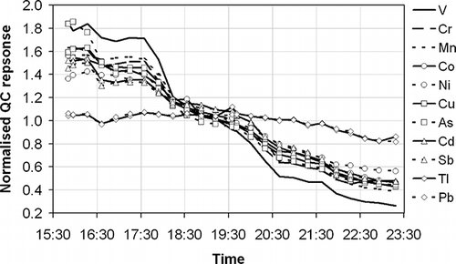
Figure 2. The analytical response of a QC sample of constant composition measured every third sample during an exemplar measurement series and normalized to the average response for each element (as indicated in the key) over the measurement period.

Figure 3. Instrumental sensitivity change observed for Co every 10 successive measurements for the measurement series displayed in . The dashed line refers to the QC limit specified in EN 14385.
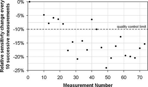
Figure 3. Instrumental sensitivity change observed for Co every 10 successive measurements for the measurement series displayed in Figure 2. The dashed line refers to the QC limit specified in EN 14385.

Figure 4. The recoveries determined from the measurement of BCR038 using standard method EN 14385 with (○) and without (•) the use of internal standards. The recoveries for Pb are overlapping. The error bars represent the overall uncertainty of the measurement at the 95% confidence interval. Both methods used the long-term drift correction procedure described in the text.
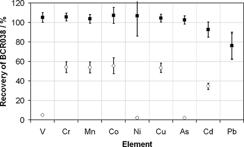
Figure 4. The recoveries determined from the measurement of BCR038 using standard method EN 14385 with (○) and without (•) the use of internal standards. The recoveries for Pb are overlapping. The error bars represent the overall uncertainty of the measurement at the 95% confidence interval. Both methods used the long-term drift correction procedure described in the text.

Figure 5. A series of measurements of Co (•) in the QC sample during a measurement series of real samples, calibration standards, and blanks, normalized to their average value during the measurement series. These measurements are fitted to a fourth-order polynomial function (black solid line; correlation coefficient: R2 = 0.996) and corrected according to Equationeq 1. The corrected data produced are also indicated (□) with the ±5% range indicated (gray dashed lines).
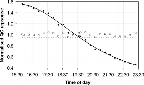
Figure 5. A series of measurements of Co (•) in the QC sample during a measurement series of real samples, calibration standards, and blanks, normalized to their average value during the measurement series. These measurements are fitted to a fourth-order polynomial function (black solid line; correlation coefficient: R2 = 0.996) and corrected according to Equationeq 1. The corrected data produced are also indicated (□) with the ±5% range indicated (gray dashed lines).

Figure 6. The corrected measured Co mass fractions as a function of the bias in the measured value, which would have been observed in the absence of correction, for the real samples considered in this study. Samples are presented as pairs (linked by the dashed lines) of sampled material (•) and their corresponding blank (○). Four exemplar pairs—a through d—are highlighted and discussed further in the text.
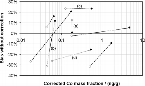
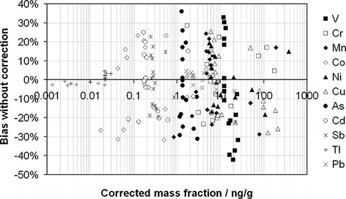
Figure 6. The corrected measured Co mass fractions as a function of the bias in the measured value, which would have been observed in the absence of correction, for the real samples considered in this study. Samples are presented as pairs (linked by the dashed lines) of sampled material (•) and their corresponding blank (○). Four exemplar pairs—a through d—are highlighted and discussed further in the text.

Table 1. The observed range of relative bias without drift correction, the average relative deviation, and the average absolute relative deviation for each of the elements measured in the real stationary-source samples displayed in

Figure 7. The observed bias without drift correction as a function of the corrected mass fraction for each element (as indicated in the key) measured in the 16 real stationary-source samples.

Figure 7. The observed bias without drift correction as a function of the corrected mass fraction for each element (as indicated in the key) measured in the 16 real stationary-source samples.

Reprints and Corporate Permissions

Please note: Selecting permissions does not provide access to the full text of the article, please see our help page How do I view content?

To request a reprint or corporate permissions for this article, please click on the relevant link below:

Academic Permissions

Please note: Selecting permissions does not provide access to the full text of the article, please see our help page How do I view content?

Obtain permissions instantly via Rightslink by clicking on the button below:

If you are unable to obtain permissions via Rightslink, please complete and submit this Permissions form. For more information, please visit our Permissions help page.