Spatio-temporal variability of polynya dynamics and ice production in the Laptev Sea between the winters of 1979/80 and 2007/08

Figures & data

Fig. 1.  Frequency of polynya occurrence during wintertime as derived from the Polynya Signature Simulation Method based on Advanced Microwave Scanning Radiometer–Earth Observing System microwave brightness temperatures, November–April, 2002–08. The following sub-areas were analysed: the eastern Severnaya Zemlya polynya (ESZ), the north-eastern Taimyr polynya (NET), the Taimyr polynya (T), the Anabar–Lena polynya (AL) and the western New Siberian polynya (WNS). Grid cell size is 6.25×6.25 km². A value of 20% means that on about 36 (out of 181) days between November and April a polynya was present in the respective grid cell. The maximum frequencies of occurrence are between 20% and 22% and are mostly found close to the fast-ice edge.

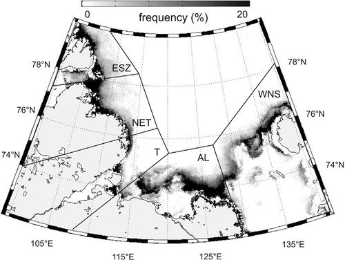
Fig. 2.  (a) Moderate resolution imaging spectroradiometer (MODIS) visible channel (background) showing the WNS polynya on 29 April 2008 1100 UTC, the Polynya Signature Simulation Method (PSSM) polynya area (thick white line) and 0.2-m ice thickness contour line as derived from MODIS thermal infrared data (29 April 2008, 2100 UTC, orange line). (b) Thin-ice thickness (0–0.5 m) as derived from the thermal infrared data, values between 0.2 and 0.5 m are subsumed to increase colour contrast for values between 0 and 0.2 m. Thick white line indicates PSSM polynya area, as in (a). (c) Surface heat loss in W/m² for the presented snapshot in combination with daily averaged reanalysis data from the National Centers for Environmental Prediction (air temperature: −13°C, 10-m wind speed: 8 m s⁻¹).

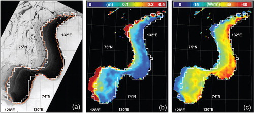
Fig. 3.  Scatterplots of November–April 2002–08 daily averages of open-water area from National Aeronautics and Space Administration Team sea-ice concentrations (sic) and Polynya Signature Simulation Method (PSSM) polynya area for the (a) western (WSL) and (b) eastern Laptev Sea (ESL). Polynomial model fits are indicated by grey lines: (a) –36.45 + 0.31x + 1.8×10⁻⁵x² (root mean square error: 676.9 km²); (b) 180.2 + 0.4x + 1.5×10⁻⁵x² (root mean square error: 1417.2 km²).

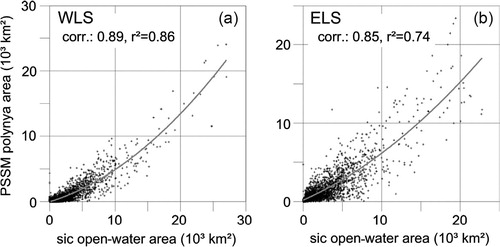
Fig. 4.  Hovmoeller diagram of the daily polynya area (November–April 1979–2008): (a) entire Laptev Sea, (b) western Laptev Sea (eastern Severnaya Zemlya polynya, north-eastern Taimyr polynya and Taimyr polynya), and (c) eastern Laptev Sea (Anabar–Lena polynya and western New Siberian polynya), as derived from the extended Polynya Signature Simulation Method (PSSM) results.

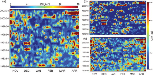
Fig. 5.  Average wintertime evolution of polyna area from monthly means including one standard deviation for (a) the western Laptev Sea and (b) the eastern Laptev Sea; linear trends of monthly averages, 1979–2008 for (c) the western and (d) the eastern Laptev Sea. In (c) and (d), black crosses indicate significance at the 90% confidence level and grey circles indicate significance at the 95% confidence level.

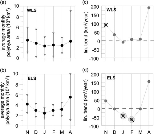
Fig. 6.  Accumulated daily winter polynya area in (a) the western Laptev Sea and (b) the eastern Laptev Sea; seasonal maxima of daily polynya area in (c) the western and (d) the eastern Laptev Sea and the number of days with open polynya (area >2000 km², >5000 km² and >10 000 km²) in (e) the western and (f) the eastern Laptev Sea. Results are for the period November–April 1979–2008. Black lines indicate linear trends significant at the 95% confidence level.

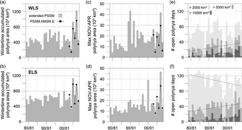
Fig. 7.  (a) Scatterplot of daily polynya area in the western (WLS) vs. eastern Laptev Sea (ELS), black dots denoting values larger than 15 000 km² (ELS) and 35 000 km² (WLS); polynya area histogram for (b) the western and (c) the eastern Laptev Sea. Bin size is 1000 km², starting with (0 to 1000 km), x-axis value represents bin (x-1000 km² to x km2).

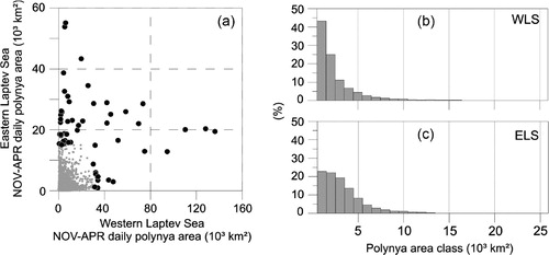
Fig. 8.  Map of relative frequency of thin-ice thickness ≤0.2 m as derived from 59 selected moderate resolution imaging spectroradiometer (MODIS) thermal infrared image data, 2002–08 (compare to Fig. 1; for thin-ice thickness retrieval see Data and methods section).

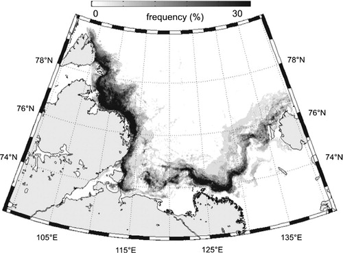
Fig. 9.  Histograms for thin-ice thicknesses (a) averaged from November to April and for the months of (b) November–December, (c) January–February and (d) March–April. Error bars indicate one standard deviation.

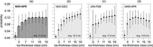
Fig. 10.  Accumulated wintertime (November–April) ice production (km³) in the Laptev Sea polynya areas. Bars indicate the standard retrieval with National Centers for Environmental Prediction (NCEP) data and an upper ice thickness of 0.20 m within the Polynya Signature Simulation Method area, split up into the eastern Laptev Sea (ELS, green) and western Laptev Sea (WLS, blue). The interannual average of 55.2 km³ is shown by a black dotted line. Modified calculations (see the section on sensitivity analysis) are indicated by lines and symbols as follows: assuming an “open-water scenario” (grey line, red downward triangle), an upper ice thickness of 0.1 m within the polynya (grey line with crosses), a reduced heat transfer coefficient of C_H=1×10⁻³ (grey line, open circles) and with modified NCEP data (2-m air temperature + 5 K and 10-m wind speed −30%: grey line, upward triangles). Black arrows mark years with significant deviation from the long-term average (positive: upward arrow; negative: downward arrow) as estimated from the relative accuracy of the ice production retrieval (see the section on sensitivity analysis).

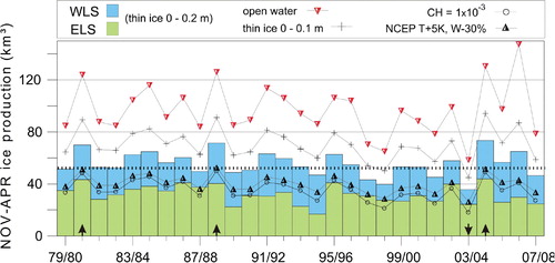
Fig. 11.  (a) Average (bars), standard deviation (black vertical lines) and maximum (triangles) of seasonal ice formation rates (m/day) for the entire Laptev Sea polynya; (b) average (bars), standard deviation (black vertical lines), maximum and minimum (triangles) of total seasonal ice production (km³) in each of the five polynya regions (eastern Severnaya Zemlya polynya [ESZ], north-eastern Taimyr polynya [NET], Taimyr polynya [T], Anabar–Lena polynya [AL] and western New Siberian polynya [WNS]) between November and April 1979/80–2007/08.

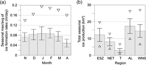
Table 1. Estimated random errors of different input parameters and their effect on the calculation of daily ice production. The thin-ice distribution error is based on the standard deviations of each class as assigned in Fig. 9. The polynya area accuracy results from comparison with moderate resolution imaging spectroradiometer (MODIS) visible and thermal infrared data.

Variable	Thin-ice distribution	Polynya area	Heat transfer coefficient CH	NCEP^a Tair	NCEP^a wind velocity
Random error	±SD	±20%	±0.5×10^−3	±2°C	±30%
▵ Ice production	±8%	±20%	±6%	±9%	±12%

^aNational Centers for Environmental Prediction, USA

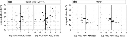
Table 2. Correlation of regional daily wintertime ice production (km³) with daily averages of National Centers for Environmental Prediction 2-m air temperature (T2m), 10-m wind speed, extended Polynya Signature Simulation method polynya area; correlation of annual wintertime ice production vs. average wintertime Arctic Oscillation Index (AO; provided by the Climate Prediction Center, National Oceanic and Atmospheric Administration, USA) and average wintertime North Atlantic Oscillation Index (NAO; provided by Climate and Global Dynamics, National Center for Atmospheric Research, USA), 1979–2008. Underlined values are based on a significant linear relationship at the 90% confidence level, bold values are significant at the 95% level.

Correlation coefficients Nov–Apr 1979–2008	T2m	Wind speed 10 m	Polynya area	AO	NAO
Ice production
Anabar–Lena Polynya	0.01	0.52	0.72	−0.19	−0.10
Western New Siberian polynya	0.21	0.51	0.85	−0.46	−0.53
Eastern Severnaya Zemlya polynya	0.19	0.45	0.84	0.40	0.36
North-eastern Taimyr polynya	0.20	0.42	0.81	0.38	0.33
Taimyr polynya	0.22	0.36	0.84	0.40	0.31

Fig. 12.  Scatterplots of annual wintertime ice production (km³) in (a) the western Laptev Sea (eastern Severnaya Zemlya, north-eastern Taimyr and Taimyr polynyas accumulated) and (b) western New Siberian polynya plotted against the average wintertime Arctic Oscillation (AO) and North Atlantic Oscillation (NAO) indices. Black triangles denote average ice production for positive and negative index values, respectively.