The intraseasonal variability of winter semester surface air temperature in Antarctica

Figures & data

Fig. 1.  of the Antarctic continent and Southern Ocean.

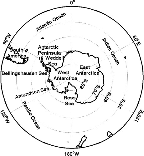
Table 1. Correlation coefficients of the time series of 2-m air temperature (April–September) during different periods for daily Reanalysis 2 data and observations from the US National Centers for Environmental Prediction.

Station	Location	Period	Days	Correlation coefficients
Amundsen–Scott	90°S	1979–2006	5124	0.603
Bellingshausen	62.2°S, 58.9°W	1979–2006	5124	0.732
Casey	66.3°S, 110.5°E	1979–2005	4941	0.692
Davis	68.6°S, 78.0°E	1979–2005	4941	0.681
Dumont d'Urville	66.7°S, 140.0°E	1979–2001	4209	0.681
Faraday	65.4°S, 64.4°W	1979–2006	5124	0.574
Ferraz	62.1°S, 58.4°W	1992–2005(no 2000)	2379	0.757
Great Wall	62.2°S, 59.0°W	1985–2005	3843	0.751
Halley	75.5°S, 26.4°W	1979–2006	5124	0.511
Macquarie	54.5°S, 158.9°E	1979–2000	4026	0.562
Mawson	67.6°S, 62.9°E	1979–2005	4941	0.726
Mirny	66.5°S, 93.0°E	1979–2006	5124	0.710
Molodeznaja	67.7°S, 45.9°E	1979–1998	3660	0.672
Neumayer	70.7°S, 8.4°W	1981–2006	4758	0.613
Novolazarevskaja	70.8°S, 11.8°E	1979–2006	5124	0.613
Rothera	67.5°S, 68.1°W	1979–2005	4941	0.600
Syowa	69.0°S, 39.6°E	1979–2004(no 1999)	4758	0.625
Vostok	78.5°S, 106.9°E	1979–2006(no 1994, 1996, 2003)	4575	0.46
Zhongshan	69.4°S, 76.4°E	1989–2005	3111	0.620

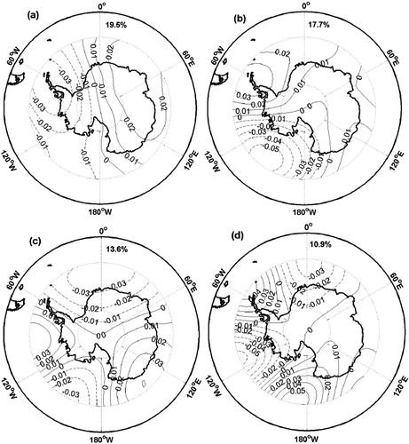
Fig. 2.  Spatial distributions of the leading four empirical orthogonal function modes of 2-m air temperature: (a) first mode, (b) second mode, (c) third mode and (d) fourth mode.

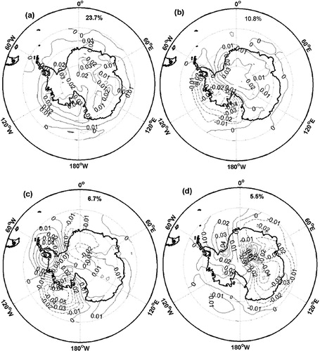
Fig. 3.  Spatial distributions of the first empirical orthogonal function mode of band-pass filtered surface pressure.

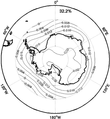
Fig. 4.  Spatial distribution of the first mode for (a) upward net longwave radiation flux and (b) 150-hPa zonal wind.

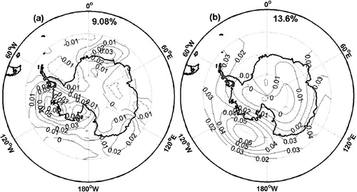
Fig. 5.  Spatial distributions of the leading four empirical orthogonal function modes for 20–90-day band-pass filtered 200-hPa streamfunction: (a) first mode, (b) second mode, (c) third mode and (d) fourth mode.

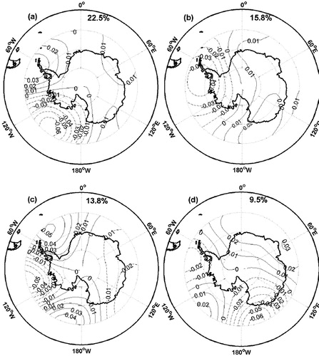
Fig. 6.  Correlations as a function of lead and lag time between time coefficients of mode 1 and mode 2 (dotted line with square markers) and between time coefficients of mode 3 and mode 4 (solid line with diamond markers).

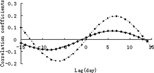
Fig. 7.  The 200-hPa 20–90-day band-pass filtered eddy streamfunction anomaly composite averaged over all (a) negative mode 1, (b) negative mode 2, (c) positive mode 1 and (d) positive mode 2. Contour interval is 1×10⁶ m² s⁻¹. Regions with values that are statistically significant at the 95% confidence level are shaded.

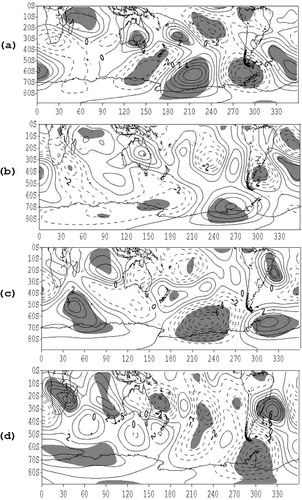
Fig. 8.  The 20–90-day band-pass filtered outgoing longwave radiation anomaly composite averaged over all (a) negative mode 1, (b) negative mode 2, (c) positive mode 1 and (d) positive mode 2. Contour interval is 1 W m⁻². Regions with values that are statistically significant at the 95% confidence level are shaded.

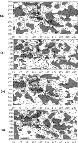
Fig. 9.  The 20–90-day band-pass filtered velocity potential anomaly composite averaged over all (a) negative mode 1, (b) negative mode 2, (c) positive mode 1 and (d) positive mode 2. Contour interval is 2×10⁵ m² s⁻¹. Regions with values that are statistically significant at the 95% confidence level are shaded.

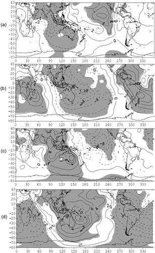
Fig. 10.  The 500-hpa 20–90-day band-pass filtered geopotential height anomaly composite averaged over all (a) negative mode 1, (b) negative mode 2, (c) positive mode 1 and (d) positive mode 2. Contour interval is 10 gpm. Regions with values that are statistically significant at the 95% confidence level are shaded.

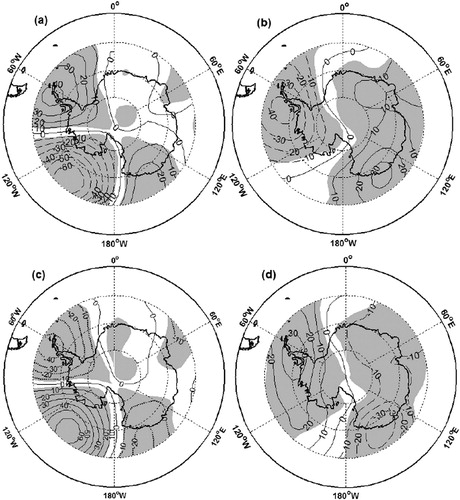
Fig. 11.  500-hpa 20–90-day band-pass filtered 10-m wind field anomaly composite averaged over all (a) negative mode 1, (b) negative mode 2, (c) positive mode 1 and (d) positive mode 2. Regions with values that are statistically significant at the 95% confidence level are shaded.

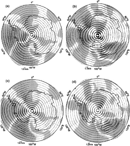
Fig. 12.  The 500-hpa 20–90-day band-pass filtered 2-m air temperature anomaly composite averaged over all (a) negative mode 1, (b) negative mode 2, (c) positive mode 1 and (d) positive mode 2. Contour interval is 0.5 °C. Regions with values that are statistically significant at the 95% confidence level are shaded.

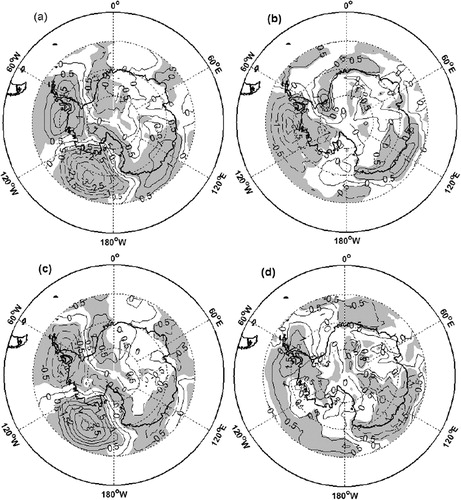
Fig. 13.  Spatial distributions of the leading four empirical orthogonal function modes for 10–20-day band-pass filtered 200-hPa streamfunction with the zonal mean removed.