Figures & data
Fig. 1 (a) The present Arctic Ocean portrayed by the International Bathymetric Chart of the Arctic Ocean (IBCAO; Jakobsson et al. Citation2008). The two major present-day surface circulation features, the Transpolar Drift and Beaufort Gyre, are shown. The Beaufort Gyre has generally two predominant regimes; one anticyclonic (black: September–May) and one cyclonic (grey: June–August) (Proshutinsky et al. Citation2002). (b) The reconstructed palaeo-bathymetry representing the early Miocene Arctic Ocean. The IBCAO grid shown in (a) was used as base data for this reconstruction (see text for further information). (c) The palaeo-bathymetric grid was translated so that the geographic position 78°N 0°E, located in the centre of Fram Strait, was moved to 30°N 0°E in order to avoid problems associated with having the North Pole included in the simulations.
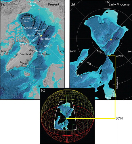
Fig. 2 Stretched grid representing the early Miocene bathymetry in the MOM4p1 simulations presented in this paper. The latitude and longitude correspond to the remapped grid.
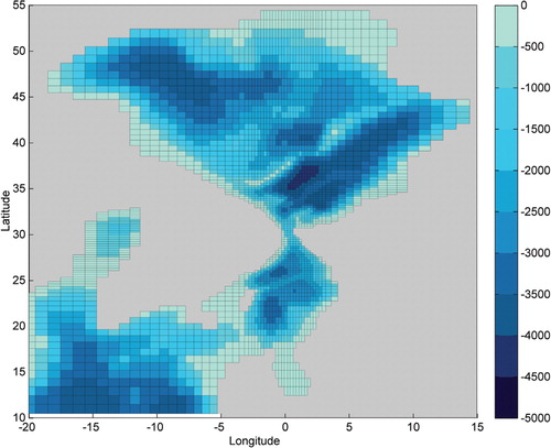
Fig. 3 The temperature and salinity reconstructions from the analysis of fish bones in ACEX 302 M0002A and M0004A. Data are obtained from Waddel & Moore (Citation2008, Table 3). The y axis represents age in millions of years before present (Mya). The black and red line represents the temperature and salinity respectively. The lower x axis is for temperature (°C) and upper x axis is for salinity (psu). The mean salinity value from the computation of Waddel & Moore (Citation2008) is plotted here. The shaded portion indicates the 28 million year long hiatus separating the early Eocene and early Miocene.
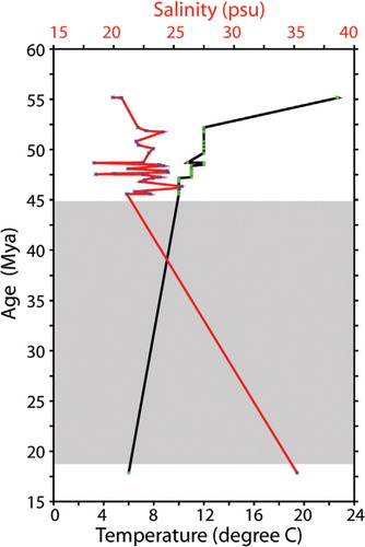
Fig. 4 Salinity (in psu) and circulation (in m/s) (a) at 5 m, (b) at 500 m and (c) at 1000 m from the Early Miocene Arctic Ocean model. The latitude and longitude correspond to the remapped model grid. The shading scale and vector lengths are separately shown for each figure.
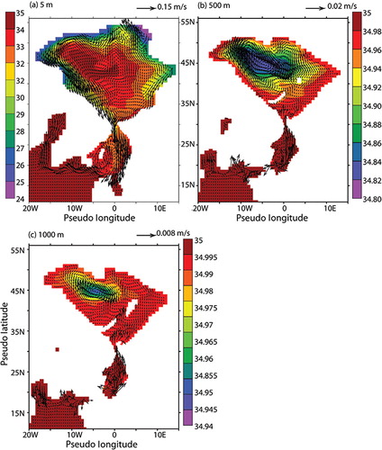
Fig. 5 The longitude-depth sections of (a) salinity (psu) and (b) meridional velocity (m/s) at the middle of Fram Strait. The longitudes correspond to the remapped model grid. Note that there are only four grid points in the strait, which presumably contributes to make the outflow broad.
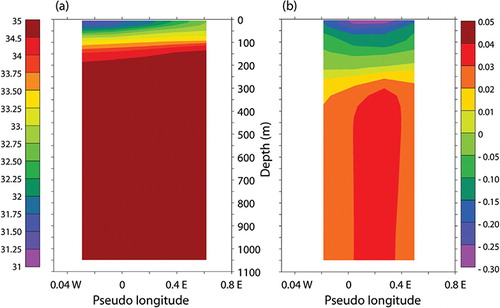
Fig. 6 Vertical distribution of salinity in the central Canada Basin simulated by the models with early Miocene (blue line) and present-day (red line) bathymetries. Below mixed layer the profiles almost overlap each other. The locations of profiles in the remapped grid are 10°W and 47°N.
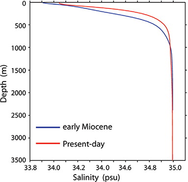
Fig. 7 Meridional overturning stream function (in Sv) computed from the model velocity field as function of (a) latitude and depth and (b) latitude and salinity. The latitudes correspond to the remapped model grid.
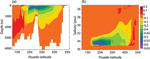
Fig. 8 Vertical variation of the tracer age in Early Miocene Arctic Ocean model, horizontal maximum age (black line) and horizontal average age (red line).
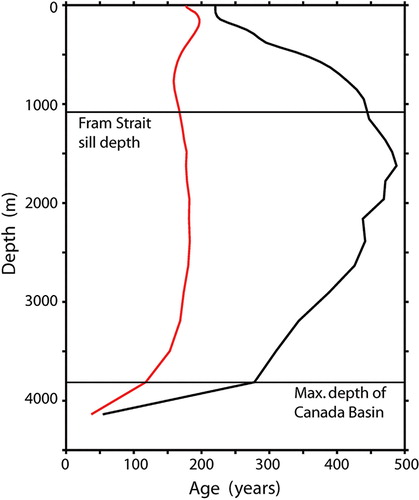
Fig. 9 Modelled tracer age (in years) at different vertical levels at (a) 5 m, (b) 500 m, (c) 1000 m and (d) 2500 m depth. The latitude and longitude correspond to the remapped model grid.
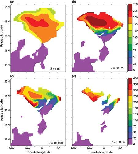
Fig. 10 The tracer age from the model (a) zonal maximum, (b) zonal minimum and (c) zonal average. The latitude corresponds to the remapped model grid. The bottom topography represents the maximum depth of ocean for the corresponding latitude.
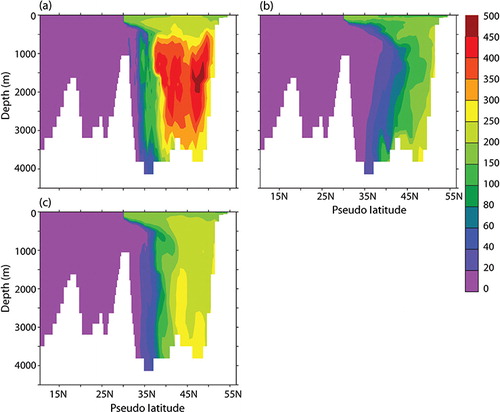
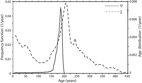
Fig. 11 The frequency function for the age distribution of particles in the Miocene Arctic Ocean, χ (dashed line) and the frequency function for the particles leaving the Arctic Ocean, ϕ (continuous line). The left y axis is for ϕ and right y axis is for χ.