Figures & data
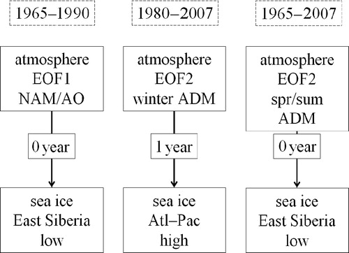
Fig. 1 Ice-cover trends and variabilities in three regions: the Beaufort–Chukchi seas, the East Siberian–Laptev seas and the Barents–Kara seas. In (a) the ice-cover time series is shown with the 3-year Hanning filter applied to the original series, shown in (b).
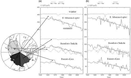
Fig. 2 The horizontal structures and time series of the first empirical orthogonal function (EOF1) for sea-level pressure (SLP) and the Northern Annular Mode/Arctic Oscillation in (a) winter (Dec.–Feb.) and (b) the average for a whole year north to 70°N. The solid lines show the time series with the 3-year Hanning filter applied on the original time series, which is indicated with dashed lines. The horizontal distributions were standardized with the average of the variance so that the time series represent standard deviations.
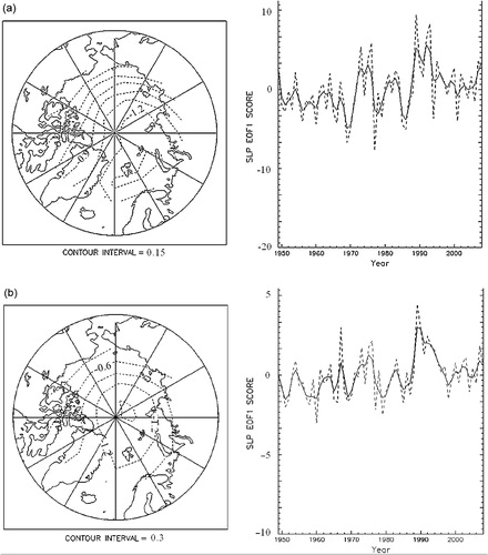
Table 1 Standard deviations of the total sea-level pressure variabilities and their first and second empirical orthogonal functions (EOFs) in four seasons—winter (Dec.–Feb.), spring (Mar.–May), summer (Jun.–Aug.) and autumn (Sep.–Nov.)—along with spring–summer (Mar.–Aug.) and the entire year. The values are spatial averages of sea-level pressure deviations (hPa): each EOF has a time series with the standard deviation shown in the table, and a spatial pattern with the average variance of unity. The analysis was carried out for the period 1950–2008. The first and second EOFs occupy about 60% and 15% of the total variance, respectively, while the amplitudes of the second EOFs are about half of the first EOFs.
Table 2 Standard deviations of the low-pass filtered and high-pass filtered Northern Annular Mode (NAM)/Arctic Oscillation (AO), Arctic Dipole Mode (ADM) and the spring–summer ADM (ADMSS), as well as the summer ice-covered areas in the three regions. The three regions are the Beaufort–Chukchi seas (BC), the East Siberian–Laptev seas (EL) and the Barents–Kara seas (BK). The original time series were de-trended and smoothed by the 3-year Hanning filter to produce the low-pass filtered time series. The differences between the de-trended original and smoothed data are defined as the high-pass filtered ones. The units are hPa for the spatial means of sea-level pressure deviations and 1102 km2 for the ice covers. The analysis was carried out for the period 1960–2008.
Table 3 (a) Correlations between the atmospheric variability and summer ice-cover variability for the low-pass filtered data, defined in , in relation to the Northern Annular Mode (NAM)/Arctic Oscillation (AO) and the Arctic Dipole Mode (ADM). The spring–summer ADM (ADMSS) is excluded, since it is minor. The three regions are the Beaufort–Chukchi seas (BC), the East Siberian–Laptev seas (EL) and the Barents–Kara seas (BK). (b) Correlations between the atmospheric variability and summer ice-cover variability for the high-pass filtered data, defined in . The correlation coefficients are shown for simultaneous cases (0-year lag) as well as the highest correlations among the lagged cases between 3 and −1-year lags, if they are higher than the simultaneous ones. Here, the lags in parentheses represent the years by which the ice cover lags from the atmosphere. Values in boldface indicate significant correlations at the 95% confidence level, where the numbers of degrees of freedom were calculated from the analysis periods divided by the zero auto-correlation timescales to be 20 for (a) and 30 for (b) during the analysis period 1960–2007. Note that the annual NAM/AO correlates very highly with the winter one at a correlation coefficient of 0.86.
Fig. 3 The horizontal structures and time series of the second empirical orthogonal function (EOF2) for sea-level pressure (SLP): (a) the Arctic Dipole Mode/Dipole Anomaly in winter; and (b) the spring–summer Arctic Dipole Mode (Mar.–Aug.).
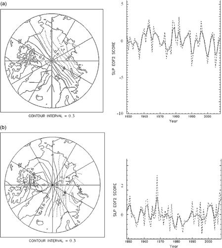
Fig. 4 (a) The sea-level pressure composite of the positive winter Arctic Dipole Mode in 1978, 1979, 1982 and 1996 and (b) the negative winter Arctic Dipole Mode in 1990, 2000 and 2005.
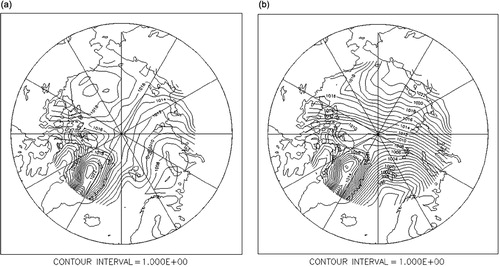
Fig. 5 (a) Summer (Jun.–Aug.) sea-ice anomalies shown as the differences between the Beaufort–Chukchi seas and the Barents–Kara seas (the latter minus the former); (b) the second empirical orthogonal function (EOF2) of the sea-level pressure (SLP) in relation to the Arctic Dipole Mode. The solid lines show the time series with the 3-year Hanning filter applied on the original time series, which is indicated with dashed lines.
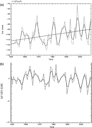
Table 4 Correlation coefficients between the winter Arctic Dipole Mode (ADM) and the summer ice cover of the Barents–Kara seas minus the Beaufort–Chukchi seas. All time series have been low-pass filtered. The period 1976–2007 was selected because the ADM shows great variability. The year values denote the lags by which the ice cover lags the ADM. Values in boldface indicate significant correlations at the 95% confidence level, where the numbers of degrees of freedom are 20 in 1960–2007 and 15 in 1976–2007.
Fig. 6 The sea-level pressure average for a whole year regressed on the summer sea ice anomalies (Barents–Kara seas minus Beaufort–Chukchi seas) with (a) zero-year and (b) one-year lags from the sea level pressure to sea ice. Here, a whole year starts in December of the previous year until November of the year in question. The ice anomalies have been normalized by their own standard deviations.
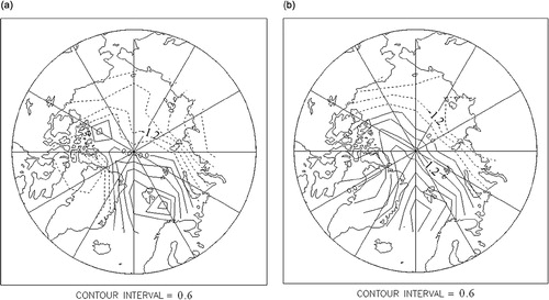
Table 5 Auto-correlation coefficients of the Northern Annular Mode (NAM)/Arctic Oscillation (AO), the Arctic Diple Mode (ADM) and the spring–summer ADM (ADMSS), where the year values denote the time differences between the time series itself and the shifted one. The original time series were already de-trended, and the analyses were carried out for the period 1960–2007. The auto-correlation coefficient is always unity at 0 lag. Values in boldface indicate significant correlations at the 95% confidence level, where the numbers of degrees of freedom are 20 for the original and low-pass filtered data and 30 for the high-pass filtered data.
Fig. 7 (a) High-pass filtered components of the atmospheric components, the Northern Annular Mode/Arctic Oscillation as the first empirical orthogonal function (EOF1), the Arctic Dipole Mode and the spring–summer Arctic Dipole Mode (Mar.–Aug.) as the second empirical orthogonal function (EOF2). (b) The summer (Jun.–Aug.) sea-ice anomalies in the three regions: the Beaufort–Chukchi seas, the East Siberian–Laptev seas and the Barents–Kara seas. The high-pass filtered components were produced by subtracting the 3-year Hanning-filtered data from the original data. Only the Northern Annular Mode/Arctic Oscillation is plotted by halving the amplitude.
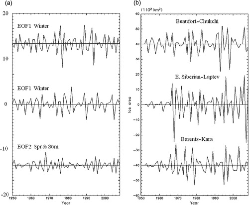
Fig. 8 Summary of relationships among the atmospheric modes and sea-ice cover. Transition in the most influential atmospheric mode is suggested from Northern Annular Mode (NAM)/Arctic Oscillation (AO) as the first empirical orthogonal function (EOF1) to Arctic Dipole Mode (ADM) as the second empirical orthogonal function (EOF2) during the 1980s, while the ADM in spring–summer (ADMSS) as EOF2 was significant for the entire period with some temporal non-homogeneity. The sea-ice features are specified to be low ice cover over the East Siberian–Laptev seas and the ice-cover difference (Atlantic sector minus Pacific sector) for the earlier and later periods, respectively. The time lags are presented for the lags from the atmospheric modes, positive NAM/AO, ADM and ADMSS, to the ice-cover anomalies.