Formation of Barents Sea Branch Water in the north-eastern Barents Sea

Figures & data

Fig. 1  Bathymetric map of the north-eastern Barents Sea and the St. Anna Trough. Stars show positions of stations obtained by the RV Professor Boyko and dots show positions of stations obtained by the RV Obva. Grey lines indicate discussed sections (see also Fig. 2).

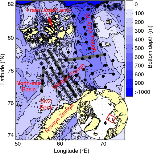
Fig. 2  Θ-S diagrams for the three sections: (a) A, (b) B and (c) C. Black lines indicate the bounds defining the different water masses: Fram Strait Branch Water (FSBW), Barents-derived Atlantic Water (bAW), Cold Deep Water (CDW) and Barents Sea Branch Water (BSBW). In (d), grey lines show positions of the sections and coloured lines show the advection paths of the different water masses. Blue lines in the Θ-S diagrams show the freezing temperature. The depth contours are similar to those in Fig. 1.

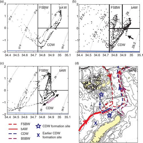
Table 1 Water mass definitions. Barents Sea Branch Water may consist of both Cold Deep Water and Barents-derived Atlantic Water and has not been given any definite bounds here.

Water mass	Temperature range (°C)	Salinity range
Atlantic Water (AW)	Θ>0	S>34.75
Fram Strait Branch Water (FSBW)	Θ>0	34.75<S<34.9
Barents-derived Atlantic Water (bAW)	Θ>0	S>34.9
Cold Deep Water (CDW)	Θ<0	S>34.75
Arctic Water	Θ<−1	34.3<S<34.7
Surface Water (SW)	Θ>−1	S<34.3

Fig. 3  Core water mass properties, represented by local maximum temperature (minimum temperature for Cold Deep Water) of the water masses discussed. The dots show the spatial distribution and the colour denote the respective core temperatures. (a) Recirculating Fram Strait Branch Water. (b) Barents-derived Atlantic Water. (c) Cold Deep Water. Depth contours similar to Fig. 1 are shown down to 500 m depth.

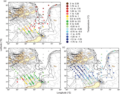
Fig. 4  Depth of water mass cores (see also Fig. 3), represented by maximum temperature (minimum temperature for Cold Deep Water) of the water masses discussed. The dots show the spatial distribution and the colour denote the respective core depths. (a) Recirculating Fram Strait Branch Water. (b) Barents-derived Atlantic Water. (c) Cold Deep Water. Depth contours similar to Fig. 1 are shown down to 500 m depth.

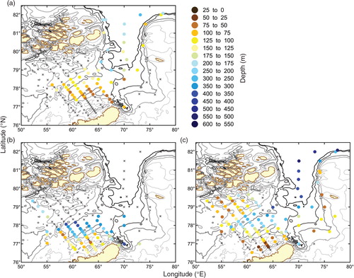
Fig. 5  Vertical sections of (a) potential temperature and (b) salinity in section C. Negative temperatures are shown by dotted lines.

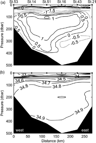
Fig. 6  Vertical sections of (a) potential temperature and (b) salinity in section B. Negative temperatures are shown by dotted lines. The blue arrow indicate dense Cold Deep Water mode in trench close to Novaya Zemlya. Inset: temperature profiles from stations 49–51 at 250–350 m depth (red box).

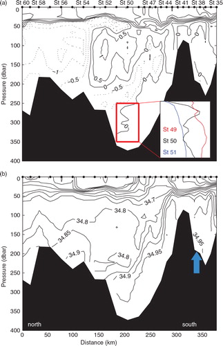
Fig. 7  Vertical section of geostrophic velocity in section B. Negative values are shown by dotted lines. Positive values toward the east.

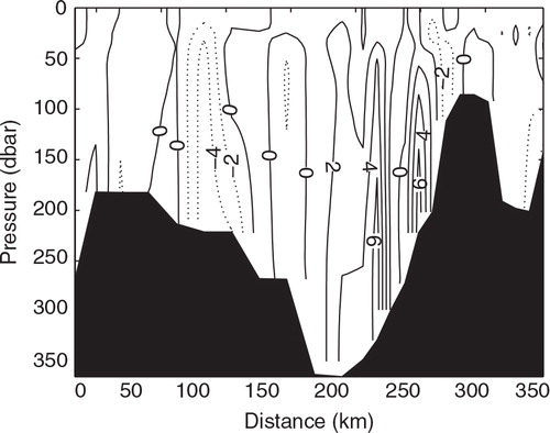
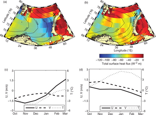
Fig. 8  Vertical sections of (a) potential temperature and (b) salinity in section A. Negative temperatures are shown by dotted lines.

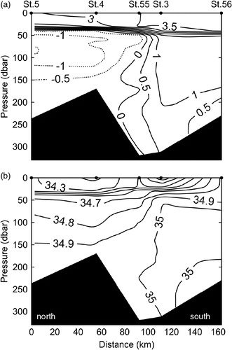
Fig. 9  Total heat fluxes between the ocean and the atmosphere (positive downwards) through the periods (a) October 1990 through March 1991 and (b) October 2007 through March 2008. X marks the sampling location on the Novaya Zemlya Bank. Lines show the mean sea level pressure (hPa) averaged over the same period. In (c) and (d), u- and v-wind velocity components and temperature at the location on the Novaya Zemlya Bank are shown.