Figures & data
Fig. 1 The location of the study area on the peninsula Brøggerhalvøya, near Ny-Ålesund, Svalbard, with boundaries of Bayelva watershed and the location of hydrological (BAY) and meteorological (W) monitoring stations. BAY is located at 78.9335 N, 11.838 E, and weather station 99910 is at 78.923 N, 11.933 E. Maps modified from Norwegian Polar Institute's online map resource, www.toposvalbard.npolar.no.
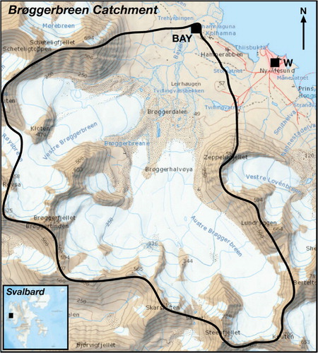
Table 1 Precipitation gradients used in the literature for calculating true precipitation in the Norwegian High Arctic. Corrections producing optimum results (marked with asterisks) were selected for the final discharge models.
Table 2 Models for estimating predicted runoff (Q p) of Bayelva, where P_JJA is areal precipitation during June–August (mm); P_JJAS is areal precipitation during June–September (mm); P_Q is daily winter precipitation causing discharge (mm); Pwinter(ngs) is areal winter snowfall on non-glacierized areas(mm); B s is summer mass balance (mm a−1); E a is evaporation (mm a−1); and C is condensation (mm a−1). The best model for calculating Q p resulting in smallest errors and the best fit to the measured discharge is presented in boldface. Models 1.0–1.2 were based on Hagen & Lefauconnier (Citation1995).
Fig. 2 Average seasonal changes by decade in (a) air temperatures and (b) Pc measured precipitation corrected for catch errors, after Killingtveit et al. (Citation2003). Winter is defined as 1 October until 31 May, while summer is 1 June until 30 September.
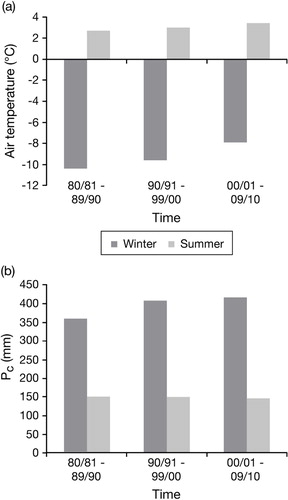
Fig. 3 Mean air temperature trends of shoulder months with their long-term averages recorded at the 99910 weather station. Data downloaded on 15 December 2011 from www.eklima.met.no.
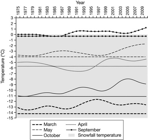
Fig. 4 The percentage of snowfall and rainfall during precipitation events recorded throughout shoulder months. Precipitation was corrected for catch errors. Precipitation in May and September in 2000 was deleted due to lack of daily precipitation records in the Eklima data set.
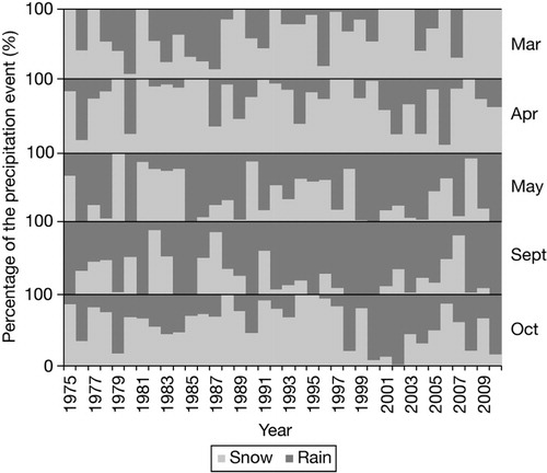
Table 3 The results of the correlation between monthly mean air temperature (T a) and precipitation in the Bayelva catchment.
Fig. 5 Winter, summer and net mass-balance record of Austre Brøggerbreen glacier. Net balance is the sum of winter and summer mass balance (data from Kohler, pers. comm. 2011).
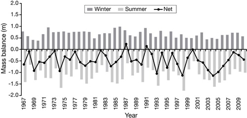
Fig. 6 Cumulative mass balance of Austre Brøggerbreen (data from Kohler, pers. comm. 2011).
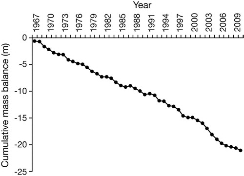
Fig. 7 Records of days with discharge of Bayelva in the Brøggerbreen catchment from 1989 until 2010: (a) commencement and cessation of runoff; (b) The duration of discharge (in days) with linear regression line showing no significant trend.
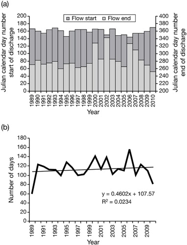
Fig. 8 Monthly specific discharge of Bayelva. Data source: Norwegian Water Resources and Energy Administration.
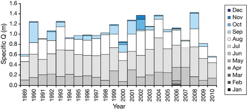
Fig. 9 The residual term in the water balance of Bayelva derived from measured and predicted runoff data.
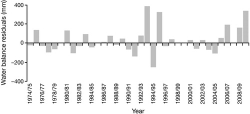
Fig. 10 Flow duration curves for Bayelva showing: (a) two periods of records 1989–1999 and 2000–10; (b) outstanding years with steeper curves of low flows than the whole period of records; and c) outstanding years with shallower curves than the whole period of records.
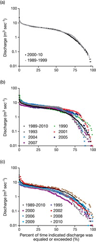
Fig. 11 Flow duration values of Bayelva during 1989–1999 and 2000–10.
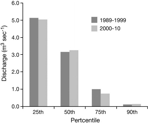
Fig. 12 Flow recession analysis of Bayelva for 1991, 2000 and 2009: (a) K1 constant values (hours) represent fast water flowpaths; (b) K2 constant values (hours) represent delayed water flowpaths.
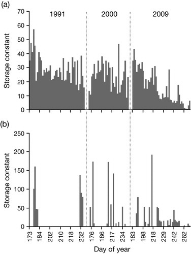
Table 4 The results of flow recession analyses of Bayelva for years representing the beginning, middle and the end of data records. K1–K3 represent different storage reservoirs.
Fig. 13 Example of ground icing after winter rainfall in the Bayelva catchment in July 2010. Photo: A. Hodson.
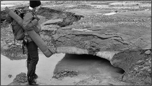
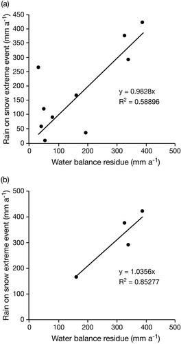
Fig. 14 The correlation between water-balance residuals (ε) and winter rain on snow events in the Bayelva catchment: (a) all hydrological years when ε was positive; (b) hydrological years when large recorded winter rain on snow events coincided with high water-balance residuals.