Summer CO₂ evasion from streams and rivers in the Kolyma River basin, north-east Siberia

Figures & data

Fig. 1  Field sample locations from 11 July to 14 August 2010. A total of 29 different sites were sampled (10 stream, 11 river and eight main stem locations), 14 of which were sampled two or more times (total n=56) spanning ca. 260 km along the Kolyma River main stem. Aquatic system types are colour coded, and streams and rivers were defined where reach length was <10 km and >10 km, respectively. Average pCO₂ for each site is represented by varying circle size.

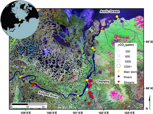
Table 1 Summary description of physical and biogeochemical characteristics of streams (<10 km reach length) and rivers (>10 km reach length) sampled in the northern Kolyma River basin during summer low-flow conditions.

		Physical characteristics^a					Biogeochemical characteristics
Inland water type	Range	Watershed (km^2)	Reach length (m)	Width (m)	Slope (°)	k ^b (cm h^−1)	Temp (°C)	DO^c (% sat.)	Cond^d (µS cm ^−1)	pH	DOC^e (mg L^−1)	Alk^f (µeq L^−1)	pCO2 ^g (µatm)
Streams (n=21)	Min	0.03	152	1	0.2	3	4.5	33	110	6.44	5.0	0.28	274
Reach length <10 000 m	Max	17	5403	19	6.5	55	19.0	114	41	7.82	21.6	1.36	9402
	Mean	5	2051	7	3.1	21	13.1	73	67	7.04	13.8	0.63	3336
Rivers (n=21)	Min	59	19 389	23	0.9	5	11.5	22	92	6.92	2.0	0.09	5
Reach length >10 000 m	Max	115 166	815 447	400	6.5	37	20.5	119	21	9.13	11.5	0.69	1010
	Mean	23 115	222 284	158	2.1	16	16.0	89	50	7.69	5.5	0.27	412
Kolyma River (n=14)	Min	424 505	2 024 530		1.6	8	11.8	88	129	7.47	3.2	0.39	123
	Max	664 119	2 319 608		1.8	28	20.1	106	66	8.22	5.3	0.81	1079
	Mean	630 029	2 232 463		1.7	17	16.1	94	88	7.75	4.4	0.56	613

^aSample size (n) only includes individual watershed once; streams (n=19), rivers (n=11), main stem (n=8).

^bBased on samples collected during summer 2011; streams (n=8), rivers (n=9), main stem (n=3).

^cDissolved oxygen.

^dConductivity.

^eDissolved organic carbon.

^fAlkalinity.

^gPartial pressure of carbon dioxide.

Fig. 2  Daily discharge of the Kolyma River (adjusted to Cherskiy, Russia, ca. 160 km downstream of the gauging station at Kolymskoye) for 2010. The grey box indicates the sampling season of this study (11 July–14 August 2010), representing summer low-flow conditions.

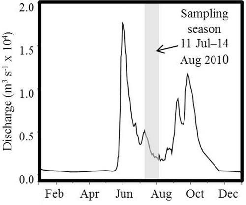
Fig. 3  Bounded study area of the lower Kolyma River basin (black box). Areal coverage of surface water for a subset of sampled rivers and streams in the Kolyma River basin determined using four different types of satellite remotely sensed imagery (Table 2). Dark blue determined from pixel value histogram reclassification and light grey predicted from the ArcGIS^TM Hydrological Extension (Table 3). Light yellow area represents the portion of the Panteleikha–Ambolikha watershed covered by GeoEye imagery (30% of the total watershed areas; Table 4). Red dots denote sampled stream locations. Lakes (light blue) were included for clarity.

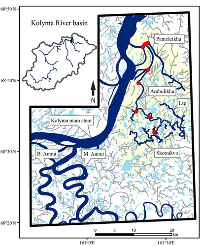
Table 2 Summary of satellite imagery used to determine water surface area within the bounded study area.

Data set	Acquisition date	Spatial resolution	Spatial coverage of study area	Availability
Orthorectified Landsat Thermatic Mapper Mosaic	N/A	14.25 m	Kolyma River main stem	National Aeronautical and Space Administration Applied Science and Technology Project Office http://zulu.ssc.nasa.gov/mrsid/
Phased Array type L-band Synthetic Aperture Radar (PALSAR)	30 July 2010	12.755 m	Large rivers (M. and B. Annui)	Alaska Satellite Facility http://www.asf.alaska.edu/
GeoEye (Panchromatic)	13 August 2009	0.48 m	Small rivers^a and streams	GeoEye http://geofuse.geoeye.com/maps/Map.aspx
Advanced Spaceborne Thermal Emission and Reflection Radar Digital Elevation Model	N/A	15 m	Length of small streams (order 1–3)	Earth Observing System Data and Information System. 2009. https://wist.echo.nasa.gov/api/

^aSmall rivers were those that PALSAR had difficulty characterizing because of their smaller size but instead could be identified in GeoEye.

Fig. 4  Comparison of (a) pCO₂ (µatm), (b) k (cm hr⁻¹), (c) CO₂ flux (g C m⁻² d⁻¹), (d) dissolved organic carbon (DOC, in mg L⁻¹) and (e) biological oxygen demand (BOD, in mg L⁻¹) among streams (<10 km reach length), rivers (>10 km reach length) and the Kolyma main stem. Box plots show range, quartiles and median. The red dashed line in (a) represents 389.3 µatm, the mean 2010 atmospheric CO₂ concentration during the sampling period (11 July–14 August 2010) and the red dashed line in (c) represents CO₂ in equilibrium with the atmosphere (values above the line indicate a CO₂ source and values below the line indicate a CO₂ sink). Average k for streams, rivers and Kolyma main stem (21.2 cm hr⁻¹, 16.2 cm hr⁻¹, 16.7 cm hr⁻¹, respectively) were used to calculate CO₂ flux.

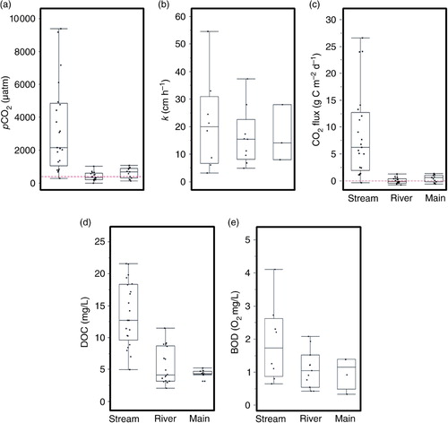
Table 3 Estimates of areal CO₂ evasion fluxes from surface waters of the northern Kolyma River bounded study area (black box in Fig. 3) during summer low-flow conditions.

Inland water type	Surface water area (km^2)	Surface water area (%)	Total study area (%)	Average pCO2 ^a (µatm)	CO2 evasion flux (g C m^−2 d^−1)	Total areal CO2 emission (10 ^6 g C d^−1)	Fractional CO2 contribution (%)
Streams (n=1034)	4.2	2.4	0.2	2860	7.00	29.5	38.3
Order 1(n=686)	1.6			3137	7.78	12.1
Order 2 (n=256)	1.5			2886	7.07	10.6
Order 3 (n=92)	1.1			2556	6.14	6.7
Small rivers (n=4)	5.6	3.2	0.3	378	−0.001	0.3	0.4
Ltp	0.3			264	−0.27	−0.1
Skotnikvo	0.9			397	0.02	0.01
Panteleikha	2.4			145	−0.50	−1.2
Ambolikha	2.0			707	0.75	1.5
Large rivers (n=2)	29.0	16.7	1.6	388	−0.005	−1.5	−2.0
Bolshoi A.	9.8			461	0.14	1.4
Malinki A.	19.2			316	−0.15	−2.9
Kolyma main stem (n=1)	134.8	77.7	7.2	547	0.35	47.2	61.3
Bounded area (1871 km^2)	173.1	100	9.3	1049	2.1	75.5	98

^aPartial pressure of carbon dioxide.

Table 4 From a watershed perspective, estimates of CO₂ evasion fluxes were scaled up to the Ambolikha–Panteleikha watershed during summer low-flow conditions.

Inland water type	Surface water area (km^2)	Surface water area (%)	Watershed area (%)	Average pCO2 (µatm)^d	CO2 evasion flux (g C m^−2 d^−1)	Total areal CO2 emission (10 ^6 g C d^−1)^e	Fractional CO2 contribution (%)
Streams (order 1–3)	2.4^a	8.7	0.13	2883	7.2	17.7	86.4
Rivers (order 4–5)	6.9^a	24.9	0.37	456	0.3	1.9	9.5
Ambolikha River	1.1^b	4.1	0.06	707	0.8	0.8	4.1
Panteleikha River	17.3^c	62.3	0.93	145	−0.5	−8.5	−41.7
Panteleikha–Ambolikha watershed (1849 km^2)	27.7	100	1.49	1048	1.9	11.9	58.3

^aThe proportion of total in known 30% of watershed (yellow area in Fig. 3) was applied to the total watershed.

^bDetermined by reclassification of GeoEye imagery.

^cLength manually measured using Orthorectified Landsat Thermatic Mapper mosaic imagery and multiplied by average width.

^dAverage partial pressure of carbon dioxide (pCO₂) from samples collected; streams (n=8), rivers (n=3), Ambolikha (n=1) Panteleikha (n=4).

^ePositive value indicates CO₂ emitted to the atmosphere and negative value indicates CO₂ absorbed by water surfaces.

Table 5 A summary of CO₂ evasion fluxes from published studies of streams, rivers and main stem locations across different geographic regions in the Northern Hemisphere. Evasion estimates were adapted from the literature to be expressed as a loss of grams of C per m² of water surface area per day. The selection includes studies for which daily evasion estimates were available (or could be readily calculated) for summer (June–August). CO₂ evasion fluxes are recorded as a range and/or a mean of samples.

	CO2 evasion flux (g C m^−2 d^−1)
Region	Watershed	Streams	Rivers	Main stem	Reference
Siberia	Kolyma River,	−0.33 to 26.56	−0.77 to 1.27	−0.62 to 1.36	This study
	Russia^a	8.59	0.01	0.46
Arctic	North Slope,	–	0.02 to 0.15	–	Kling et al. (1991)
	Alaska		0.09
Boreal	Eastman River, Canada	3.12	0.39	0.19	Teodoru et al. (2009)
Temperate	Brocky Burn,	0.26 to 45.88	–	–	Hope et al. (2001)
	Scotland	–

^a Calculated from all field-based samples; see Table 1.

Kling G.W, Kipphut G.W, Miller M.C. Arctic lakes and streams as gas conduits to the atmosphere: implications for tundra carbon budgets. Science. 1991; 251: 298–301.

 PubMed Web of Science ®Google Scholar

Teodoru C.R, del Giorgio P.A, Prairie Y.T, Camire M. Patterns in pCO2 in boreal streams and rivers of northern Quebec, Canada. Global Biogeochemical Cycles. 2009; 23: 2012.

 Web of Science ®Google Scholar

Hope D, Palmer S.M, Billett M.F, Dawson J.J.C. Carbon dioxide and methane evasion from a temperate peatland stream. American Society of Limnology and Oceanography. 2001; 46: 847–857.

 Web of Science ®Google Scholar