Automated ice-sheet snowmelt detection using microwave radiometer measurements

Figures & data

Fig. 1  Scatterplots and regression lines for the Antarctic data from 1 January 2009 to 29 April 2009: (a) data from the Special Sensor Microwave/Imager (SSM/I) 19-GHz horizontal channel and (b) data from the SSM/I 37-GHz vertically polarized channel.

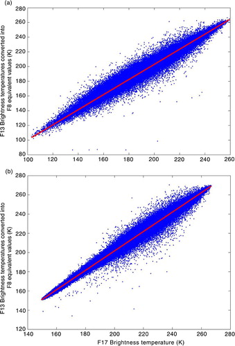
Table 1 Regression coefficients for data adjustments between different sensors in Antarctica.

Conversion	Slope	Intercept	Correlation coefficient
SSM/I^a F-17 37-Ghz vertical to SSM/I F-8 37-Ghz vertical	1.008	−1.17	R>0.99
SSM/I F-17 19-Ghz horizontal to SSM/I F-8 19-Ghz horizontal	1.0286	−3.0094	R>0.99

^aSpecial Sensor Microwave/Imager.

Fig. 2  Cross-gradient polarization ratio (XPGR) values at the Wilkins Ice Shelf area (from 1978 to 2010).

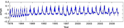
Fig. 3  Cross-gradient polarization ratio (XPGR) histogram and optimal threshold at the Wilkins Ice Shelf area (from 1978 to 2010). The red asterisk is the unsupervised XPGR threshold (−0.0293) obtained by the melt signal adaptation method.

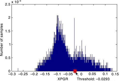
Fig. 4  Segmentation line of the optimal threshold at the Wilkins Ice Shelf area (from 1978 to 2010). The red line is the unsupervised Cross-gradient polarization ratio (XPGR) threshold (−0.0293) obtained by the melt signal adaptation method.

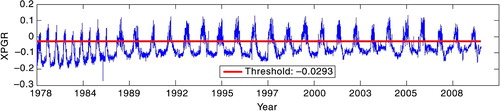
Fig. 5  Flowchart of modified cross-gradient polarization ratio (XPGR) detection method. Scanning Multichannel Microwave Radiometer is abbreviated to SMMR and Special Sensor Microwave/Imager to SSM/I.

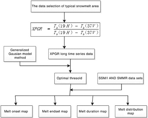
Fig. 6  Two optimal thresholds obtained from a bimodal Gaussian distribution model (BG) and a generalized Gaussian model (GG).

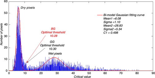
Fig. 7  Flowchart of the modified ice-sheet snowmelt detection method based on wavelet transformation. Scanning Multichannel Microwave Radiometer is abbreviated to SMMR and Special Sensor Microwave/Imager to SSM/I.

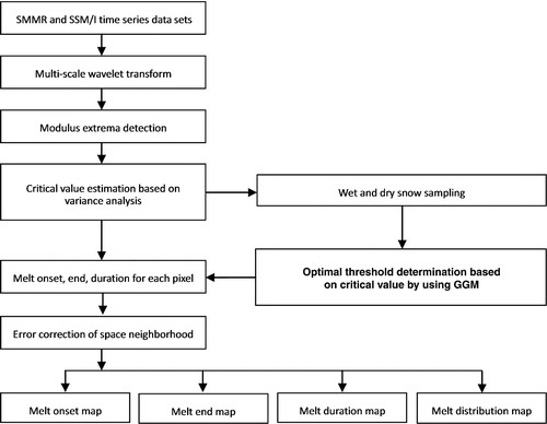
Fig. 8  The threshold determination based on cross-gradient polarization ratio (XPGR) value in the Greenland study area. The solid blue line represents the XPGR values from 1988 to 1995, the red line is the XPGR threshold (−0.0158) obtained by Abdalati & Steffen's (1997) method, and the light blue line is the unsupervised XPGR threshold (−0.0152).

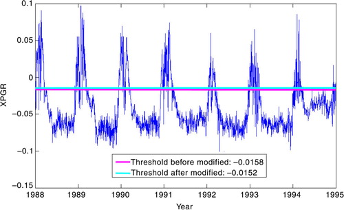
Fig. 9  Ice-sheet snowmelt distribution of the modified cross-gradient polarization ratio (XPGR) detection method and the XPGR method on 2 August 1996: (a) the result of the XPGR method; (b) the result of the modified XPGR method.

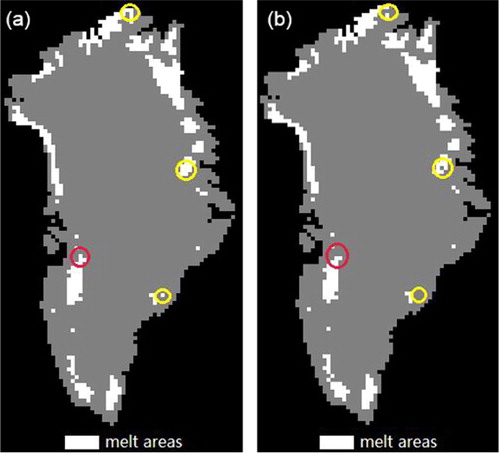
Fig. 10  Ice-sheet snowmelt distribution during 2007–08 derived from the two optimal thresholds: (a) the bimodal Gaussian distribution model optimal threshold; (b) the generalized Gaussian model automatic threshold.

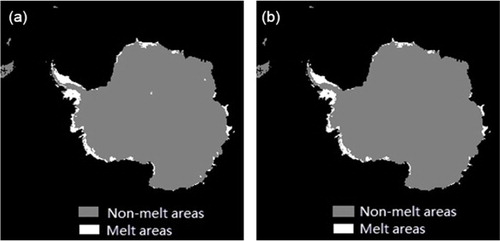
Fig. 11  Ice-sheet snowmelt detection results obtained from the modified wavelet transformation method in Antarctica, 2007–08: (a) melt onset; (b) melt end; (c) melt duration.

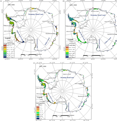
Table 2 Automatic weather stations.

Station name	Latitude/longitude	Elev.	Dates	Days	Min.	Max.	SD
Larsen Ice Shelf	66.90S/60.60W	50 m	07/02/83–01/01/86	2390	36.46 m	49.78 m	1.6874
	66.97S/60.55W		01/01/86–01/02/99
–	66.949S/60.897W	–	01/02/99–02/01/04	–	–	–	–
	67.012S/61.550W		02/01/04–01/01/07
	67.012S/61.550W		01/01/07–
Butler Island	72.20S/60.34W	91 m	01/03/86–25/01/89	2449	−14.80 m	95.36 m	16.83
	72.21S/60.16W		25/01/89–11/01/97
	72.21S/60.17W		11/01/97–11/01/00
–	72.207S/60.160W	–	11/01/00–22/12/03	–	–	–	–
	72.206S/60.170W		02/02/05–02/02/11
	72.206S/60.170W		02/02/11–
Bonaparte Point	64.78S/63.06W	8 m	05/01/92–09/03/94	1761	−35.10 m	311.72 m	77.97
	64.78S/63.07W		09/03/94–23/12/96
–	64.778S/63.067W	–	23/12/96–14/03/08	–	–	–	–
	64.778S/63.067W		14/03/08–20/11/09
	64.778S/63.067W		20/11/09–
Amery G3	70°53′31′′S/69°52′21′′E	84 m	1999–	1931	95.20 m	104.08 m	1.84

Table 3 Quantitative snowmelt detection results (in %), applying two methods in four areas.

Automatic weather station	Snowmelt detection method	P TP ^a	P FP b	P TN ^c	P FN ^d	CDR^e	Priori TPR^f	Posterior TPR^g
Bonaparte Point	Wavelet	55.03	4.49	12.66	27.83	67.69	66.42	92.46
	XPGR^h	32.14	3.35	13.80	50.71	45.94	38.79	90.56
Butler Island	Wavelet	6.7	15.03	71.87	6.41	78.56	51.09	30.83
	XPGR	4.08	14.56	72.02	9.34	76.09	30.38	21.87
Larsen Ice Shelf	Wavelet	22.51	13.14	51.38	12.97	73.89	63.44	63.15
	XPGR	26.16	20.81	45.59	7.44	71.75	77.86	55.70
Amery G3	Wavelet	4.97	9.01	83.43	2.59	88.40	65.75	35.56
	XPGR	5.58	20.42	71.90	2.09	77.49	72.73	21.48

^aThe number of melt days that were correctly detected.

^bThe number of non-melt days that were incorrectly detected as “melt” days.

^cThe number of non-melt days that were correctly detected.

^dThe number of melt days that were incorrectly detected as “non-melt” days.

^eCorrect detection rate, the ratio between the number of correct detection results and the total number of detection results.

^fPriori true positives rate, the ratio between the number of correctly detected “melt” results and the number of temperature data above 0°C.

^gPosterior true positives rate, the ratio between the number of correctly detected “melt” results and the number of detected “melt” results.

^hCross-gradient polarization ratio.

Abdalati W, Steffen K. Snowmelt on the Greenland Ice Sheet as derived from passive microwave satellite data. Journal of Climate. 1997; 10: 165–175.

 Web of Science ®Google Scholar