Influence of winter sea-ice motion on summer ice cover in the Arctic

Figures & data

Fig. 1  The ice edge on 10 September for the nine years of 2003–2011.

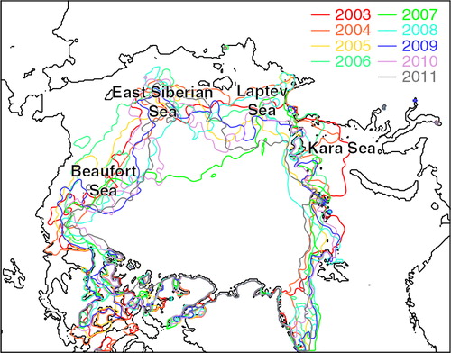
Fig. 2  Comparison of drifting buoy motion and Microwave Scanning Radiometer—Earth Observing System (AMSR-E) satellite-derived ice motion. (a) Scatterplot of ice drift speed derived from AMSR-E versus buoy speed based on 4868 daily data, for horizontal direction of (c). b) Same as (a) but for vertical direction. Dotted lines are regression lines defined by the first principal component of plots. (c) Trajectories of 30 buoys (bold lines) and those of particles calculated from the AMSR-E derived ice velocity (thin lines) during one year from 1 December to 30 April 2009–2010 (blue lines) and 2010–11 (red lines).

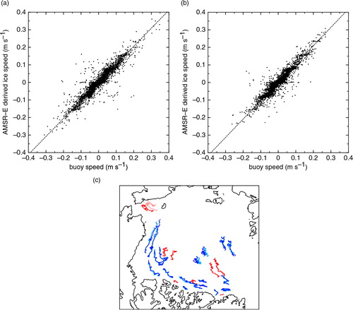
Fig. 3  Distribution of migrating particles for (a) 1 December 2004, (b) 20 January 2005, (c) 10 March 2005, (d) 30 April 2005, (e) 1 December 2007, (f) 20 January 2008, (g) 10 March 2008 and (h) 30 April 2008, which are first arrayed over the ice-covered area on 1 December and are moved based on the Microwave Scanning Radiometer—Earth Observing System satellite-derived daily-ice velocity.

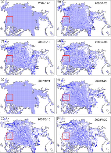
Fig. 4  Bold lines indicate the fraction of sea ice existing since before 1 December and the temporal evolution of the number of particles within that part of the Beaufort Sea bounded by the red squares shown in Fig. 3 for 2005 and 2008 The unit of the particle number is converted to ice area (km²) by multiplying by 37.5×37.5, under the assumptions that each particle represents a 37.5×37.5 km of area with 100% ice concentration and that ice melting during December and April is negligible. Thin lines show the corresponding total sea-ice area within the same region calculated from the daily-ice concentration.

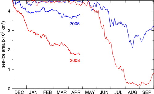
Fig. 5  Standard deviation of (a) sea-ice area on 10 September (IA9) and (b) number of particles (NP4) on 30 April for 108 domains in 10⁴ km².

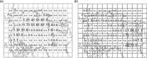
Fig. 6  (a) Correlation coefficient between the number of particles on 30 April migrated from 1 December (NP4), and the total ice area on 10 September (IA9) of the same year for 108 domains, based on the nine years’ data. Panels below are scatterplots of IA9 versus NP4 for domains shown by (b) blue, (c) red and (d) green rectangles. Dotted lines in these panels show regression lines defined by the first principal component of plots.

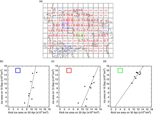
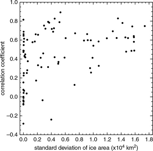
Fig. 7  Scatterplot of the derived correlation coefficient shown in Fig. 6a versus standard deviation of total ice area on 10 September (IA9) shown in Fig. 5a for the 108 domains.