Figures & data
Table 1 A summary of five stability functions used for stable conditions.
Fig. 1 The fourth Chinese National Arctic Research Expedition (CHINARE 2010) ice station drift indicated by the line (A→B), along with the Surface Heat Budget of the Arctic Ocean (SHEBA) ice camp drift (X→Y). The CHINARE 2010 drift lasted from 12 to 19 August 2010, and the SHEBA drift started in October 1997 and ended in October 1998.
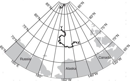
Fig. 2 Hourly mean (a) air pressure, (b) surface and air temperature, (c) relative humidity (with respect to saturation over water), (d) wind speed and (e) radiation measurements made during the fourth Chinese National Arctic Research Expedition. The downward and upward shortwave radiations are indicated by Sd and Su, respectively, and the downward and upward longwave radiations are indicated by Ld and Lu, respectively. Rn represents the net radiation.
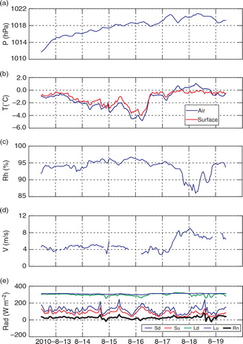
Fig. 3 The surface temperature (T s) in spring (March—May 1998, green dots), summer (June—August 1998, red dots), autumn (October 1997 and September—October 1998, orange dots) and winter (December 1997—February 1998, blue dots) plotted as a function of the air–surface temperature difference (ΔT=T a−T s) using data from the Surface Heat Budget of the Arctic Ocean (SHEBA) 20-m tower. Data from the fourth Chinese National Arctic Research Expedition (CHINARE 2010) ice station are represented by black dots. T a is the air temperature measured at a height of 2.2 m for SHEBA and 2 m for CHINARE 2010.
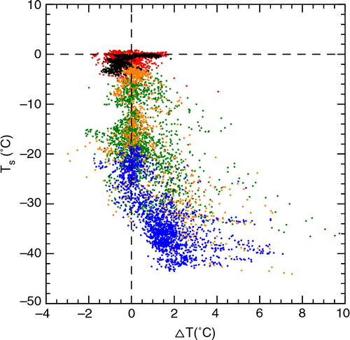
Fig. 4 Intercomparison of the dimensionless gradient functions for (a) wind speed φ m (ζ) and (b) potential temperature φ h (ζ) for stable stratification. B71, HDB88, BH91, Z98 and CB05 denote the functions proposed by Businger et al. (Citation1971), Holtslag & de Bruin (Citation1988), Beljaars & Holtslag (Citation1991), Zeng et al. (Citation1998) and Cheng & Brutsaert (Citation2005), respectively.
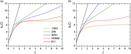
Fig. 5 Intercomparison of the stability functions for (a) wind speed ψ m (ζ) and (b) potential temperature ψ h (ζ) for stable stratification. B71, HDB88, BH91, Z98, and CB05 denote the functions proposed by Businger et al. (Citation1971), Holtslag & de Bruin (Citation1988), Beljaars & Holtslag (Citation1991), Zeng et al. (Citation1998) and Cheng & Brutsaert (Citation2005), respectively.
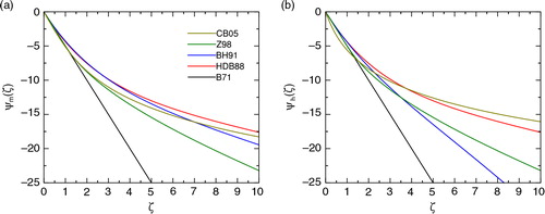
Fig. 6 Theoretical relationships between the Deacon number for wind speed profile D m and gradient Richardson number R i for (a) R i less than 0.5 and (b) R i greater than 0.1.
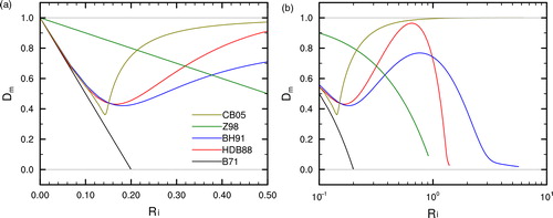
Fig. 7 Theoretical relationships between the Deacon number for potential temperature profile D h and gradient Richardson number R i for (a) R i less than 0.5 and (b) R i greater than 0.1.
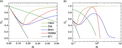
Table 2 A comparison of five sets of φ m and φ h functions in the limit of very stable stratification. The laminar case is a theoretically expected limit.
Fig. 8 Hourly (a) wind stresses, (b) sensible heat (SH) fluxes and (c) latent heat (LH) fluxes from Surface Heat Budget of the Arctic Ocean (SHEBA) 20-m tower observations and bulk algorithms plotted as a function of the air–surface potential temperature difference Δθ (Δθ=θ a−θ s) in 0.5K bins on the SHEBA 20-m tower. θ a is the potential temperature calculated at the lowest tower level (2.2 m).
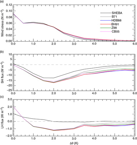
Fig. 9 The number of hourly observations for all the 5 levels (2.2 m, 3.2 m, 5.1 m, 8.9 m, and 18.2 m or 14 m) at the Surface Heat Budget of the Arctic Ocean 20-m tower in each of the 0.5K Δθ bins between −4 and+12K.
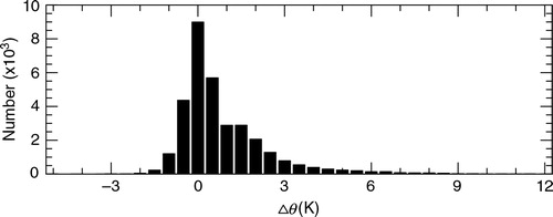
Fig. 10 Monthly means of (a) wind stress, (b) sensible heat (SH) flux and (c) latent heat (LH) flux measured at the 20-m Surface Heat Budget of the Arctic Ocean (SHEBA) tower along with the bulk fluxes from BCC_CSM, ECMWF, CESM and CESM_const during the SHEBA year, with positive fluxes being upward.
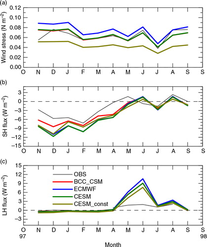
Fig. 11 Hourly mean (a) wind stress, (b) sensible heat flux and (c) latent heat flux during the period of the fourth Chinese National Arctic Research Expedition. The in situ measurements are indicated by blue lines, and the algorithm fluxes derived from BCC_CSM are indicated by red lines.
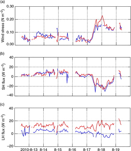
Table 3 Evaluation of the wind stresses (t), sensible heat flux (SH) and latent heat flux (LH) of the four model algorithms using the hourly the Surface Heat Budget of the Arctic Ocean (SHEBA) 20-m tower observations. Shown are the biases, that is, the differences between computed and observed medians; the root-mean square error (RMSE) between computed and observed values. M obs is the mean value of the observed flux. Numbers in boldface denote the smallest bias and RMSE. The values in the parentheses indicate the bias and RMSE as a percentage of the observed mean. “Winter” is from October 1997 to 14 May 1998 and 15 September 1998 to the end of the SHEBA deployment in early October 1998. “Summer” is from 15 May to 14 September 1998.
Fig. 12 Scatterplots of friction velocity u * measured at the fourth Chinese National Arctic Research Expedition ice station (green circles) and the portable automated mesonet station named Atlanta (red dots) and modelled with the bulk algorithms of (a) the new algorithm proposed in this article (NEW), (b) the Beijing Climate Centre Climate System Model (BCC_CSM), (c) the European Centre for Medium-Range Weather Forecasts model (ECMWF) and (d) the Community Earth System Model (CESM). In each panel, the black dashed line is 1:1. The blue line is the best fit through the data, taken as the bisector of y-vs.-x and x-vs.-y least-square fits (e.g., Andreas Citation2002).
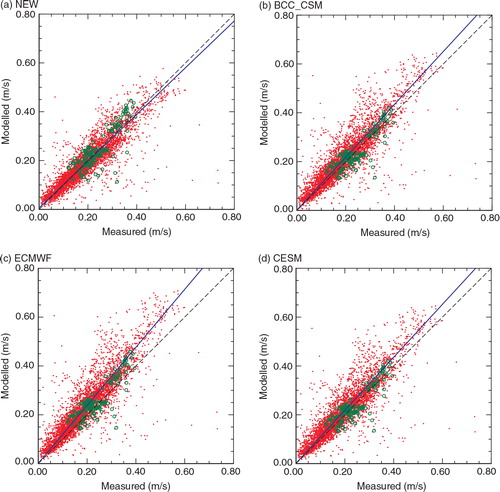
Fig. 13 Scatterplots of the sensible heat flux H s at the fourth Chinese National Arctic Research Expedition ice station (green circles) and the portable automated mesonet station named Atlanta (red dots) and modelled with the bulk algorithms of (a) the new algorithm proposed in this article (NEW), (b) the Beijing Climate Centre Climate System Model (BCC_CSM), (c) the European Centre for Medium-Range Weather Forecasts model (ECMWF) and (d) the Community Earth System Model (CESM). In each panel, the black dashed line is 1:1. The blue line is the best fit through the data taken as the bisector of y-vs.-x and x-vs.-y least-square fits (e.g., Andreas Citation2002).
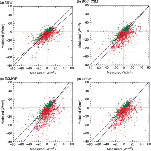
Fig. 14 Scatterplots of the latent heat flux H l at the fourth Chinese National Arctic Research Expedition ice station (green circles) and on the 20-m tower (red dots) and modelled with the bulk algorithms of (a) the new algorithm proposed in this article (NEW), (b) the Beijing Climate Centre Climate System Model (BCC_CSM), (c) the European Centre for Medium-Range Weather Forecasts model (ECMWF) and (d) the Community Earth System Model (CESM). In each panel, the black dashed line is 1:1. The blue line is the best fit through the data taken as the bisector of y-vs.-x and x-vs.-y least squares fits (e.g., Andreas Citation2002).
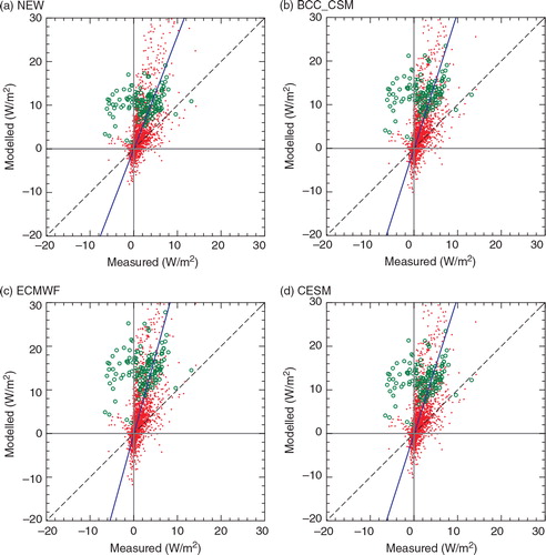
Table 4 Performance of the four algorithms depicted in Figs. 12–14 for the u * and H s data from the Atlanta ice station and for H l from the 20-m tower in winter (October 1997 to 14 May 1998 and 15 September 1998 to the end of the Surface Heat Budget of the Arctic Ocean project deployment in early October 1998) and summer (15 May to 14 September 1998). u *,obs, H s,obs and H l,obs are the mean of the observed values. The values in parentheses indicate the bias and root-mean square error (RMSE) as a percentage of the observed mean.