Figures & data
Fig. 1 Inset shows the location of the Antarctic Peninsula. Main figure is a regional map of the western Antarctic Peninsula study area including multibeam bathymetry from the International Bathymetric Chart of the Southern Ocean (Arndt et al. Citation2013), created using Fledermaus software (Quality Positioning Systems BV, Zeist, Netherlands). The location of the Antarctic Circumpolar Current (ACC) and Bransfield Current are shown. Four study sites with published records that data in this study are compared to are as follows: (1) Domack et al. (Citation2001); (2) Heroy et al. (Citation2008); (3) Michalchuk et al. (Citation2009); and (4) Milliken et al. (Citation2009) and Majewski et al. (Citation2012). This study (5) is the site of core JPC-24, collected during NBP0703.
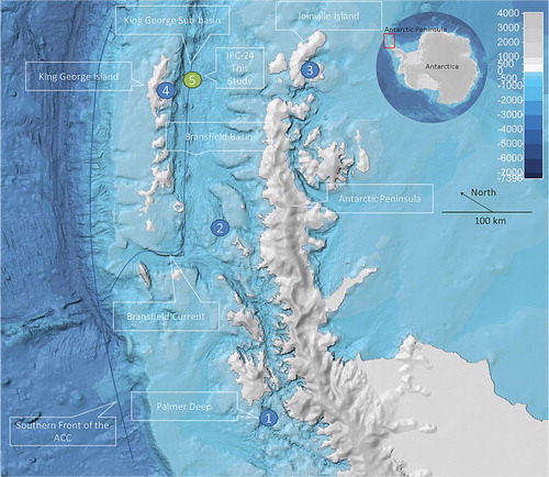
Fig. 2 Bathymetry of the Bransfield Basin. Location of Fig. 3 is shown as a red line with core locations as a green circle. Map created using GeoMapApp (Carbotte et al. Citation2007).
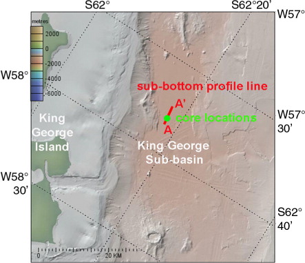
Fig. 3 Chirp 3.5 kHz sub-bottom profile, y-axis is depth and x-axis is distance. Vertical exaggeration in the bathymetric profile is approximately 40. Inset: changes in the core lithology (JPC-24) correlate with acoustic reflection surfaces. The location is shown in Fig. 2. Inset: core lithology represented by colours, where green is clayey mud, orange is clay, grey is sand–gravel and mottling represents abundant organic matter. Vertical bars are grain size, from left to right: clay, sand, gravel.
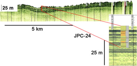
Table 1 Dates were calibrated using Calib v.6.0 software and using the marine 04.14c calibration curve that incorporates a 350–400 years correction (Stuiver et al. Citation2005). A marine reservoir ΔR of 700 years was added, making the total marine reservoir correction about 1100 years.
Fig. 4 Age model for the radiocarbon dates, constructed by linear interpolation, showing 1σ error bars. Because 1950 AD is equivalent to 0 cal yr BP, the age model uses negative values on the x axis to reach 2007 AD (−57 cal yr BP). The calculated sedimentation rate, based on a linear interpretation from the origin to 22 m at 3559 cal yr BP, is 0.6 cm/yr.
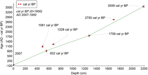
Fig. 5 Grain size (sand, silt, clay percentages), multi-sensor core logger data (density and magnetic susceptibility), pebble count, elemental and isotopic data (total organic carbon and nitrogen (wt.%), δ13C, δ15N (‰) and the C/N atomic ratio) for units and super-units throughout JPC-24 plotted by age (cal yr BP).
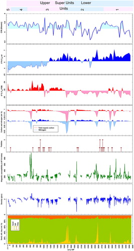
Fig. 6 Atomic carbon and nitrogen ratio of organic matter. The correlation coefficient for the best-fit line is 0.99. The traditional Redfield Ratio has a slope between 3 and 8 and here the best-fit line has a slope of 5.1.
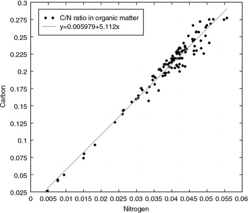
Fig. 7 Three-dimensional plot of δ13C and C/N ratio. The highest δ13C values occur in the youngest parts of the core.
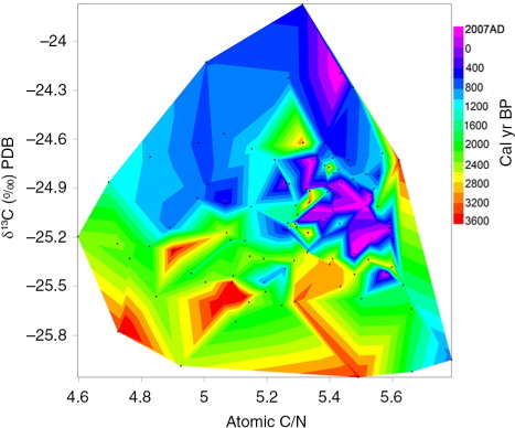
Fig. 8 Total organic carbon and nitrogen mass accumulation rate, δ13C and δ15N values cross-plot with best-fit lines, correlation coefficients for nitrogen 0.48 and carbon 0.41, standard deviation of 0.69 and 0.36, respectively.
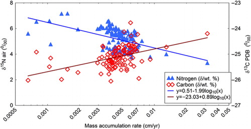
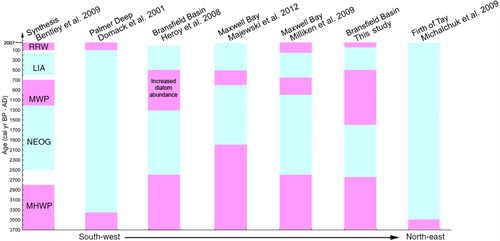
Fig. 9 Summary showing the warm (pink) and cold (blue) periods defined in other studies and compared to this study. Bentley et al. (Citation2009) presented a summary including onshore and offshore work but the timings of the changes are uncertain and are shown as gaps. The other six columns are marine records organized geographically from south-west to north-east. Terms are abbreviated as follows: Recent Rapid Warming (RRW); Little Ice Age (LIA); Medieval Warm Period (MWP); Neoglacial (NEOG); Mid-Holocene Warm Period (MHWP).