Verification of a new NOAA/NSIDC passive microwave sea-ice concentration climate record

Figures & data

Fig. 1  Spatial distribution of: (a) monthly Climate Data Record (CDR) concentrations, (b) local standard deviation (SD), (c) monthly NASA Team (NT) concentrations and, (d) concentration difference between monthly Bootstrap (BT) and NT estimates for the Northern Hemisphere in September 2000. The units are percent concentration.

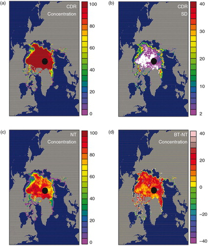
Fig. 2  Spatial distribution of: (a) monthly Climate Data Record (CDR) concentrations, (b) local standard deviation (SD), (c) monthly NASA Team (NT) concentrations and, (d) concentration difference between monthly Bootstrap (BT) and NT for the Southern Hemisphere in September 2000. The units are percent concentration.

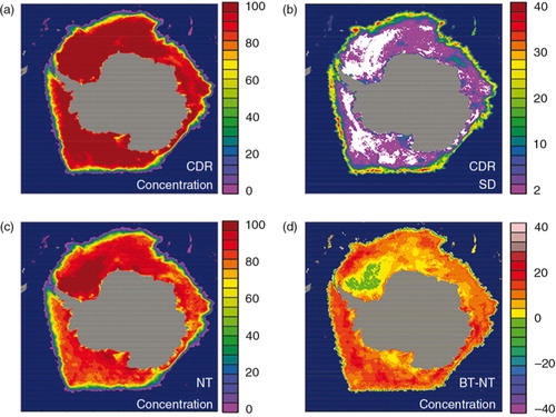
Table 1 Summary of the characteristics of the National Oceanic and Atmospheric Administration Climate Data Record (CDR) concentration and the comparison combined Goddard Space Flight Center (GSFC) concentration. Main differences between the two are shown in boldface.

Description	CDR	GSFC
Source TBs^a	RSS^b-based polar stereo gridded	RSS-based polar stereo gridded
RSS TB version	Ver. 4, ver. 6	Ver. 2, ver. 4
Algorithms	NT, BT^c	NT, BT
Algorithm processing location	NSIDC ^d	GSFC
Ice edge definition	BT≥10%	BT≥10%
Concentration value	Greater of NT, BT	Greater of NT, BT
Automated weather, coast filters	Yes	Yes
Interpolation to fill missing data?	No	Yes
Manual quality control	No	Yes
Period of data	July 1987–December 2007	October 1978–December 2007

^aBrightness temperatures.

^bRemote Sensing Systems Inc.

^cNASA Team, Bootstrap.

^dNational Snow and Ice Data Center.

Fig. 3  Number of missing grid cells over the full grid (136 192 grid cells total) for each day, 2 January 1988–31 December 2007 in (a) the Northern Hemisphere and (b) the Southern Hemisphere. The y axis is logarithmic. Values >100 000 represent days with no data (i.e., all grid cells are missing).

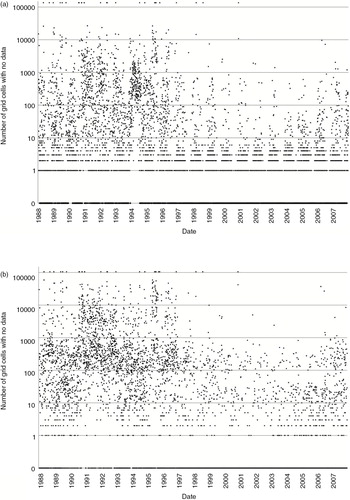
Table 2 Number of days over 1 January 1988–31 December 2007 in each hemisphere with missing grid cells in each range. There were no days with >40 000 missing grid cells other than days with no data.

No. of missing grid cells	Northern Hemisphere	Southern Hemisphere
0	2615	3936
1–10	2693	551
11–100	865	854
101–1000	747	1370
1001–10 000	292	402
10 001–20 000	31	65
20 001–30 000	6	28
30 001–40 000	0	25
No data	45	45

Fig. 4  Spatial distribution of 20 years (1988–2007) (a) mean and (b) standard deviation (SD) of monthly sea-ice concentrations from the National Oceanic and Atmospheric Administration Climate Data Record (CDR), Goddard Space Flight Center (GSFC), Bootstrap (BT) and NASA Team (NT) algorithms in the Northern Hemisphere. Units are fraction ice concentration (0–1). Grid cells with sea-ice concentrations less than 0.15 (15%) are not included in the calculations.

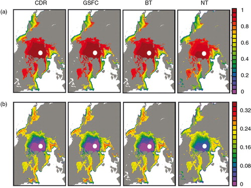
Fig. 5  Spatial distribution of 20 years (1988–2007) (a) mean and (b) standard deviation (SD) of monthly sea-ice concentration from the National Oceanic and Atmospheric Administration Climate Data Record (CDR), Goddard Space Flight Center (GSFC), Bootstrap (BT) and NASA Team (NT) algorithms in the Southern Hemisphere. Units are fraction ice concentration (0–1). Grid cells with sea ice concentrations less than 0.15 (15%) are not included in the calculations.

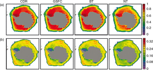
Fig. 6  Spatial distribution of bias (mean difference) and root mean square difference (RMSD) of monthly sea ice concentration anomaly between: (a), (e) the National Oceanic and Atmospheric Administration Climate Data Record (CDR) and Goddard Space Flight Center (GSFC); (b), (f) CDR and Bootstrap (BT); (c), (g) CDR and NASA Team (NT); and (d) and (h) BT and NT in the Northern Hemisphere. Note that the scale factor for (c), (d), (g) and (h) is five times larger than that of (a), (b), (e) and (f). Units are in fraction concentration (0–1). Grid cells with sea-ice concentrations less than 0.15 (15%) are not included in the calculations.

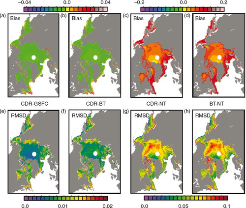
Fig. 7  Spatial distribution of bias (mean difference) and root mean square difference (RMSD) of monthly sea ice concentration anomaly between: (a), (e) the National Oceanic and Atmospheric Administration Climate Data Record (CDR) and Goddard Space Flight Center (GSFC); (b), (f) CDR and Bootstrap (BT); (c), (g) CDR and NASA Team (NT); and (d) and (h) BT and NT in the Southern Hemisphere. Note that the scale factor for (c), (d), (g) and (h) is five times larger than that of (a), (b), (e) and (f). Units are in fraction concentration (0–1). Grid cells with sea-ice concentrations less than 0.15 (15%) are not included in the calculations.

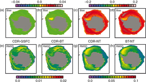
Fig. 8  Time series of monthly Northern Hemisphere the National Oceanic and Atmospheric Administration Climate Data Record (CDR) (a) extent and (b) area for 1988–2007 (thick solid lines: blue for March and red for September) and difference between CDR and Goddard Space Flight Center estimates (dashed lines). Note the different y axis scales for the extent/area (left axis) and the differences (right axis). The dotted lines are linear trends.

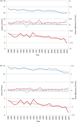
Fig. 9  Times series of monthly Southern Hemisphere National Oceanic and Atmospheric Administration Climate Data Record (CDR) (a) extent and (b) area for 1988–2007 (thick solid lines: blue for March and red for September) and difference between CDR and Goddard Space Flight Center estimates (dashed lines). Note the different y axis scales for the extent/area (left axis) and the differences (right axis). The dotted lines are linear trends.

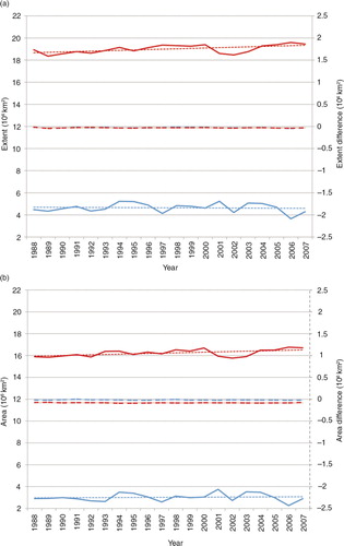
Fig. 10  The scatter diagram of monthly sea ice extents (10⁶ km²) from monthly National Oceanic and Atmospheric Administration Climate Data Record (CDR) and (a) Goddard Space Flight Center, (b) NASA Team (NT) and (c) Bootstrap (BT) data. The left column of diagrams is for the Northern and the right is for the Southern Hemisphere.

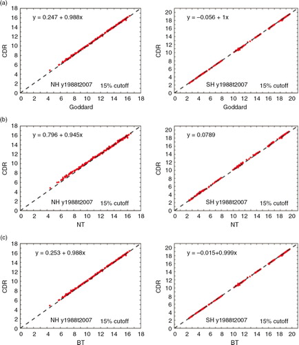
Table 3 Confusion matrix for comparison of National Oceanic and Atmospheric Administration Climate Data Record (CDR) and Goddard Space Flight Center (GSFC) sea-ice extent. a and d represent correct “forecasts” counts for a given time period, while b and c are incorrect, using GSFC as the “correct” estimate.

Class type	GSFC sea ice	GSFC no-ice
CDR sea ice	a Correct ice	b False ice
CDR no-ice	c False no-ice	d Correct no-ice

Table 4 A summary of results of confusion matrix for September and March for the Northern (NH) and Southern (SH) hemispheres for the 20-year period from 1988 to 2007. The mean, minimum and maximum percentages for each month are provided as well as the overall range of percentages.

	a (%)			b (%)			c (%)			d (%)
	Correct CDR ice^a			False CDR ice^b			False CDR no-ice^c			Correct CDR no-ice^d
Class Mon/HH	Mean	Min	Max	Mean	Min	Max	Mean	Min	Max	Mean	Min	Max
Mar/NH	36.2	33.9	38.0	0.27	0.14	0.47	0.007	0.002	0.015	63.5	61.7	65.9
Sep/NH	14.5	9.23	17.8	0.57	0.18	1.13	0.003	0.000	0.015	84.9	82.1	89.8
Mar/SH	7.97	6.34	9.25	0.02	0.009	0.04	0.000	0.000	0.002	92.0	90.7	93.6
Sep/SH	37.2	35.9	38.4	0.014	0.006	0.05	0.002	0.000	0.004	62.8	61.6	64.1
Range	6.34–38.4			0.006–1.13			0.00–0.015			61.6–93.6

^{a, b, c, d}The states of the confusion matrix, as provided in Table 3.

Fig. 11  Confusion matrix diagrams for the (a) and (b) Northern Hemisphere and (c) and (d) Southern Hemisphere in (a) and (c) March and (b) and (d) September. GSFC refers to the sea ice fields produced by Goddard; CDR are the climate data record fields. Note that different scales are used in the shaded areas. The circled “x” marks the value of the percentage occurrence of year 1988 for the event, with adjacent empty circles moving clockwise representing subsequent years through 2007.

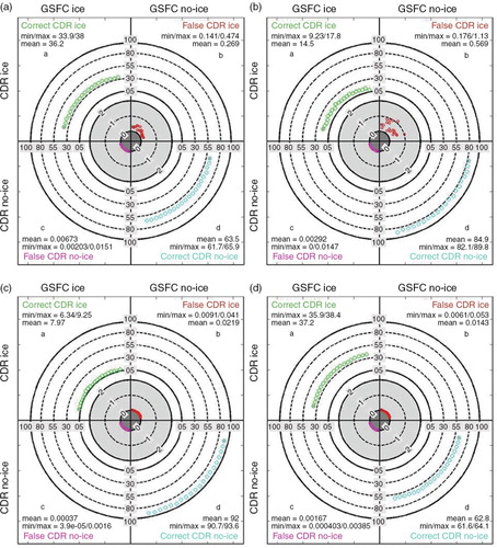
Fig. 12  Temporal evolution of (a) and (b) accuracy, (c) and (d) precision, (e) and (f) false/incorrect classification of the National Oceanic and Atmospheric Administration Climate Data Record (CDR parameter in (a), (c) and (e) March and (b), (d) and (f) September for the Northern Hemisphere for the period of years 1988–2007. A 15% concentration cut-off is used to delineate ice and no-ice classification and missing grid cells are not included. The mean, minimum and maximum monthly values over the entire 1988–2007 period are given at the top of each plot.

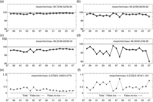
Fig. 13  Temporal evolution of (a) and (b) accuracy, (c) and (d) precision, (e) and (f) false/incorrect classification of the National Oceanic and Atmospheric Administration Climate Data Record (CDR) parameter in (a), (c) and (e) March and (b), (d) and (f) September for the Southern Hemisphere for the period of years 1988–2007. A 15% concentration cut-off is used to delineate ice and no-ice classification and missing grid cells are not included. The mean, minimum and maximum monthly values over the entire 1988–2007 period are given at the top of each plot.

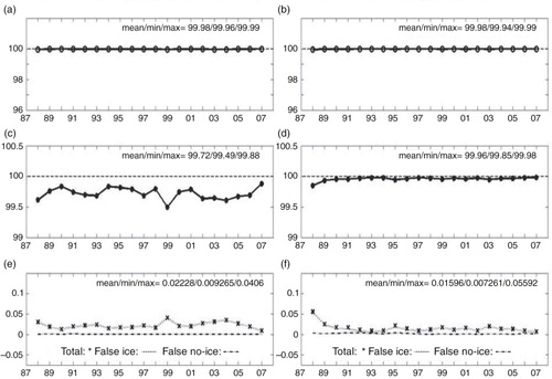
Table 5 Monthly sea-ice extent trend estimates (in km²) over 1988–2007 for the National Oceanic and Atmospheric Administration Climate Data Record (CDR) and the difference between CDR and Goddard Space Flight Center (GSFC) for the Northern and Southern Hemispheres.

	Northern Hemisphere		Southern Hemisphere
Month	CDR trend	CDR–GSFC trend (SD)	CDR trend	CDR–GSFC trend (SD)
January	−63 500	−2100 (49 000)	−5300	−200 (20 400)
February	−55 300	−1700 (98 700)	+13 500	[phone])
March	−57 100	−2600 (68 300)	−5400	−300 (9900)
April	−52 000	−1300 (48 500)	+4100	[phone])
May	−28 700	−1500 (53 100)	+2400	−1800 (40 500)
June	−37 400	−3700 (87 900)	+17 700	−1200 (21 900)
July	−76 500	−3800 (67 400)	+22 500	+300 (8000)
August	−82 200	−5700 (102 500)	+11 600	[phone])
September	−98 700	−400 (111 300)	+35 400	−300 (6600)
October	−78 800	[phone])	+29 900	[phone])
November	−83 400	[phone])	+18 000	[phone])
December	−57 200	[phone])	+8500	−5700 (121 800)

Fig. 14  Northern Hemisphere CDR ice area for (a) March and (b) September from the National Oceanic and Atmospheric Administration Climate Data Record (CDR; red), Bootstrap (blue) and NASA Team (green), in solid lines. Dashed lines are the difference between CDR and Goddard Space Flight Center. Dotted lines are linear trends.

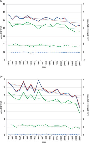
Fig. 15  Southern Hemisphere CDR ice area for (a) March and (b) September from the National Oceanic and Atmospheric Administration Climate Data Record (CDR; red), Bootstrap (blue) and NASA Team (green), in solid lines. Dashed lines are the difference between CDR and Goddard Space Flight Center. Dotted lines are linear trends.

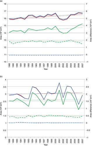
Table 6 Monthly sea-ice extent trend estimates (in km²) over 1988–2007 for the National Oceanic and Atmospheric Administration Climate Data Record (CDR) and the difference between CDR and NASA Team (NT) for the Northern and Southern Hemispheres.

	Northern Hemisphere		Southern Hemisphere
Month	CDR trend	CDR–NT trend (SD)	CDR trend	CDR–NT trend (SD)
January	−59 500	−600 (94 900)	−1100	0 (97 800)
February	−49 600	−2300 (89 700)	+9500	[phone])
March	−49 500	−7000 (101 800)	−5200	[phone])
April	−37 200	−3200 (95 500)	+5500	[phone])
May	−30 200	[phone])	+2100	[phone])
June	−51 300	[phone])	+20 100	[phone])
July	−71 500	−3000 (129 800)	+26 300	[phone])
August	−83 700	−7500 (159 500)	+11 400	[phone])
September	−91 700	−16 600 (178 700)	+29 800	+300 (6900)
October	−95 000	[phone])	+24 700	[phone])
November	−72 600	[phone])	+15 700	[phone])
December	−68 275	[phone])	+15 000	−3500 (107 600)

Table 7 Monthly sea ice extent trend estimates (in km²) over 1988–2007 for the National Oceanic and Atmospheric Administration Climate Data Record (CDR) and the difference between CDR and Bootstrap (BT) for the Northern and Southern Hemispheres.

	Northern Hemisphere		Southern Hemisphere
Month	CDR trend	CDR–BT trend (SD)	CDR trend	CDR–BT trend (SD)
January	−59 500	−500 (26 500)	+700	−200 (12 800)
February	−49 600	−100 (68 800)	+100	+500 (7000)
March	−49 500	−700 (38 400)	−700	−300 (11 800)
April	−37 200	−700 (40 100)	−200	+900 (9000)
May	−30 200	−800 (42 300)	−1900	−1800 (43 200)
June	−51 300	−1000 (52 600)	−1900	−1200 (25 100)
July	−71 500	−3300 (41 700)	+600	[phone])
August	−83 700	−2900 (60 400)	+600	[phone])
September	−91 700	[phone])	−100	−300 (6900)
October	−95 000	[phone])	+200	[phone])
November	−72 600	[phone])	+900	[phone])
December	−68 275	[phone])	−8000	−5700 (108 600)