Turbulent fluxes of momentum and heat over land in the High-Arctic summer: the influence of observation techniques

Figures & data

Fig. 1  (a) The archipelago of Svalbard north of mainland Norway. (b) The location of Adventdalen on the island of Spitsbergen. (c) The measuring site (image published courtesy of the Norwegian Polar Institute).

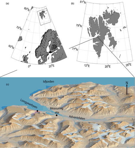
Fig. 2  Overview of daily meteorological parameters: (a) temperature at 2 m (T ₂) in 2010 and (b) in 2011; (c) relative humidity at 2 m (RH ₂) in 2010 and (d) in 2011; (e) wind speed at 10 m (U ₁₀) in 2010 and (f) in 2011.

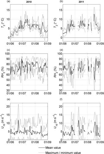
Table 1 Monthly overview of mean meteorological parameters at 2 and 10 m: temperature (T ₂ and T ₁₀), relative humidity (RH ₂ and RH ₁₀) and wind speed (U ₂ and U ₁₀); mean sensible heat fluxes from the eddy covariance method (H _S,ECM ), the gradient method (H _S,GM ), the bulk method (H _S,BM ) and the modified bulk method (H _S,BM,Mod ), and mean latent heat flux from the gradient method (H _L,GM ). Numbers in brackets indicate the percentage of data available.

	June		July		August
	2010	2011	2010	2011	2010	2011
T 2 (°C)	3.7 (100)	4.9 (100)	6.7 (100)	6.9 (65)	5.0 (100)	6.7 (77)
T 10 (°C)	3.5 (100)	4.7 (100)	6.6 (100)	6.8 (65)	5.0 (100)	6.7 (77)
RH 2 (%)	72 (100)	72 (100)	77 (100)	75 (65)	75 (100)	76 (77)
RH 10 (%)	73 (100)	72 (100)	79 (100)	76 (65)	77 (100)	77 (77)
U 2 (m s^−1)	4.1 (100)	3.5 (100)	4.1 (100)	5.0 (65)	3.0 (100)	3.9 (77)
U 10 (m s^−1)	4.8 (100)	4.2 (100)	4.9 (100)	6.1 (65)	3.7 (100)	5.0 (100)
H S,ECM (W m^−2)	–	42.1 (36)	37.6 (60)	24.3 (64)	25.7 (60)	11.0 (67)
H S,GM (W m^−2)	31.6 (85)	26.0 (86)	27.4 (61)	10.5 (75)	13.9 (64)	−3.1 (67)
H S,BM (W m^−2)	–	97.5 (79)	109.7 (64)	79.7 (66)	67.9 (69)	54.3 (70)
H S,BM Mod (W m^−2)	–	65.9 (79)	74.6 (64)	54.6 (66)	46.2 (69)	41.8 (70)
H L,GM (W m^−2)	−3.9 (85)	19.7 (86)	−17.7 (61)	−8.8 (75)	−16.2 (64)	−16.3 (67)

Fig. 3  Overview of daily means of radiation parameters: (a) the four components of radiation in 2010 and (b) in 2011; (c) net radiation (R _N ) in 2010 and (d) in 2011; and (e) albedo (α) in 2010 and (f) in 2011.

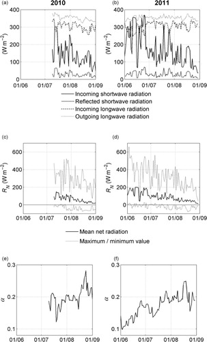
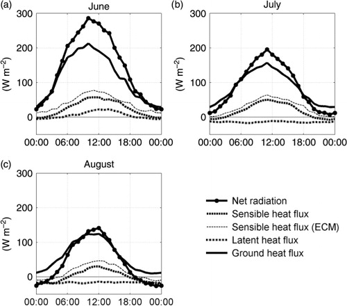
Fig. 4  Daily radiation budget for (a) June, (b) July and (c) August.

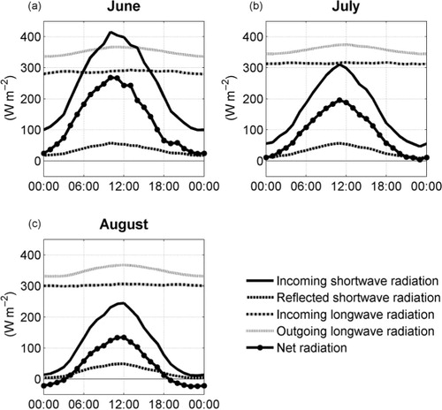
Fig. 5  Comparison of the bulk Richardson number (Ri _B ) and z/L: (a) Ri _B between 2 and 10 m; (b) Ri _B between the surface and 10 m.

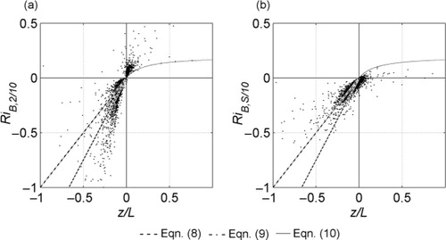
Fig. 6  The aerodynamic roughness length (z ₀) calculated for near neutral values, in (a) and (c) using sonic anemometer data (−0.025<z/L<0.025) with Eqn. 11 and in (b) and (d) using slow-response measurements (−0.025<Ri _B,2/10<0.025) with Eqn. 12. (a) and (b) show z ₀ as a function of wind direction (WD) and (c) and (d) as a function of the wind speed at 10 m (U ₁₀), where median values for each 2.5 m s⁻¹ are also shown (large filled circles).

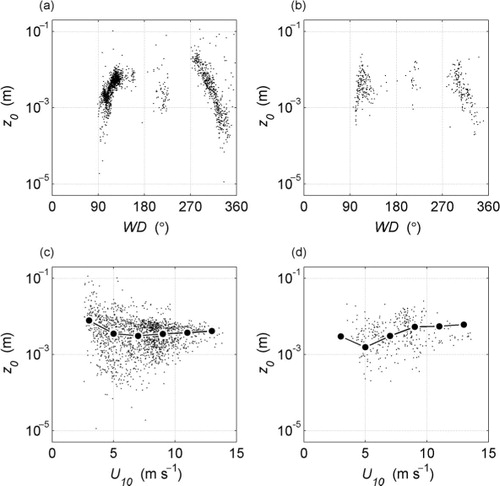
Fig. 7  Comparison of different methods to calculate momentum flux (τ) and sensible heat flux (H _s ): (a) and (b) plot of the eddy covariance method (ECM) against the gradient method (GM); (c) and (d) plot of the ECM against the bulk method (BM); (e) and (f) plot of the ECM against a modified BM, as described in the text.

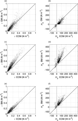
Fig. 8  Time series for 2010 and 2011: (a) and (b) show the sensible heat flux (H _s ) calculated with the eddy covariance method and (c) and (d) with the gradient method. In (e) and (f) the latent heat flux (H _L ) from the gradient method is shown.

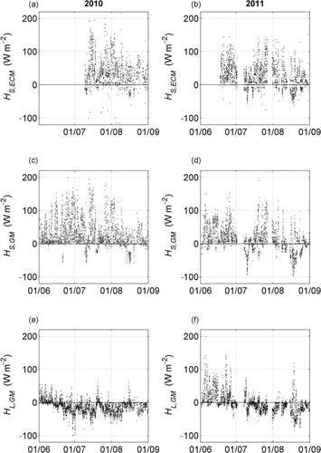
Fig. 9  Daily surface energy budget (SEB) for (a) June, (b) July and (c) August. For comparison, the sensible heat flux from the eddy covariance method (ECM) is shown.