Modelling snow ice and superimposed ice on landfast sea ice in Kongsfjorden, Svalbard

Figures & data

Table 1 Numerical values of model parameters and constants in high-resolution thermodynamic snow and sea-ice model (HIGHTSI).

Abbreviation	Parameter/constant	Value
c i	Specific heat of sea ice	2093 J kg^−1 K^−1
c s	Specific heat of snow	2093 J kg^−1 K^−1
ρ i	Density of sea ice	910 kg m^−3
ρ s	Initial density of snow	330 kg m^−3
ρ w	Density of sea water	1020 kg m^−3
ρ sui	Superimposed ice density	850 kg m^−3
ρ slush	Slush density	920 kg m^−3
T f	Freezing point temperature of seawater	−1.8°C
L f	Specific latent heat of freezing	0.33×10^6 J kg^−1

Fig. 1  Map of Kongsfjorden, Svalbard, with the four measurement sites in 2004. The Svalbard Archipelago is shown in the inset.

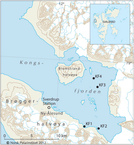
Fig. 2  Observed in situ mean (a) snow depth, (b) sea-ice thickness and (c) freeboard, and their mean standard deviation (vertical bars) from 23 January to 21 May 2004. In (b), zero refers to sea-ice surface and the blue curve indicates the ice bottom.

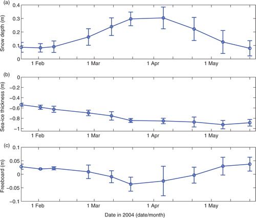
Fig. 3  (a) Air temperature, (b) wind speed and direction and (c) precipitation (mm water equivalent [WE]) recorded at Sverdrup Station in Ny-Ålesund, and (d) derived snow thickness from solid precipitation from 23 January to 21 May 2004, assuming snow density of 330 kg m⁻² and taking a temperature threshold of 0.5°C.

Fig. 4  Calculated snow density (coloured symbols) based on individual snow and ice thicknesses and freeboard measurements at sites KF1–KF4 according to Archimedes’ Principle. The calculated mean snow density (black line with open circles), the polynomial (n=2) fit (red line) in a least-squares sense of mean snow density and the parameterized snow density in accordance with Anderson (1976) (blue line) are also shown.

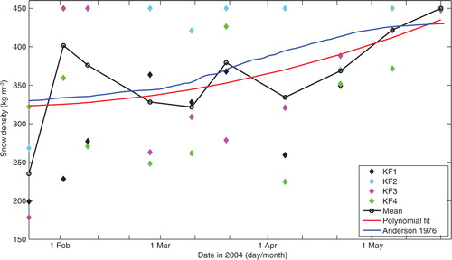
Table 2 Configurations of high-resolution thermodynamic snow and sea-ice model (HIGHTSI) experiments.

Experiment run	Parameters
Ref (Reference run)	ρ s ^a (initial)=330 kg m^−3; ρ s calculated according to the parameterization of Anderson (1976); F w ^b=2 W m^−2; Snow input=solid precipitation
S1	Ref set-up, but ρ s is derived from in situ data
S2	S1 set-up, snow input=85% solid precipitation
S3	S2 set-up, albedo scheme (Flato & Brown 1996)
F1	Ref set-up, but F w =5 W m^−2
F2	Ref set-up, but F w =10 W m^−2
F3	Ref set-up, but F w time-dependent; F w =2, if h i ^c≤0.6; F w =h i ×15−7, if 0.6≤h i ≤1; and F w =8, if h i >1

^a ρ _s is the snow density. ^b F _w is the oceanic heat flux. ^c h _i is the ice thickness.

Fig. 5  The observed mean snow, freeboard and ice thickness (black open circles) compared to high-resolution thermodynamic snow and sea-ice model (HIGHTSI) modelled results in model runs Ref (black lines), S1 (red lines), S2 (green lines) and S3 (blue lines).

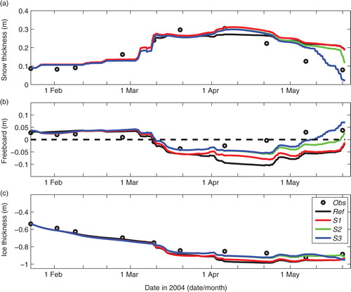
Table 3 Bias, root mean square error (RMSE) and correlation coefficient of simulated snow thickness, freeboard and ice thickness compared to observations.

	Snow thickness (h s )			Freeboard (f b )			Ice thickness (h i )
Model runs	Bias (cm)	RMSE (cm)	Corr. coef.	Bias (cm)	RMSE (cm)	Corr. coef.	Bias (cm)	RMSE (cm)	Corr. coef.
Ref	2.2	5.5	0.83	−3.0	5.5	0.54	4.7	6.3	0.98
S1	3.0	5.9	0.84	−2.2	4.5	0.54	4.5	5.7	0.99
S2	1.7	4.4	0.90	−0.8	2.9	0.68	2.6	3.6	0.99
S3	0.5	4.1	0.90	−0.1	2.7	0.80	2.7	4.0	0.98

Fig. 6  The modelled snow slush thickness due to (a) ocean flooding events and (b) surface and subsurface melting, sleet or rainfall in the high-resolution thermodynamic snow and sea-ice model (HIGHTSI) model experiments Ref, S1, S2 and S3.

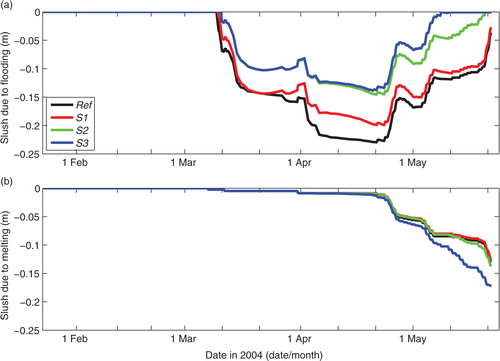
Fig. 7  Modelled ice growth from ice bottom using different oceanic heat fluxes in the high-resolution thermodynamic snow and sea-ice model (HIGHTSI) runs: Ref (Fw=2 W m⁻²), F1 (Fw=5 W m⁻²), F2 (Fw=10 W m⁻²) and F3 (time-dependent).

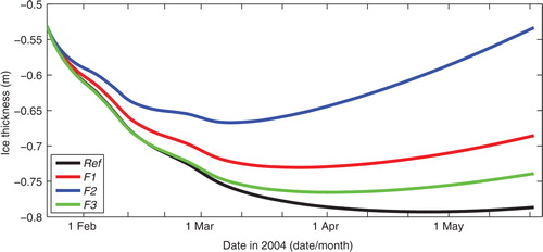
Fig. 8  The seasonal (December–May) mean air temperature and precipitation for a climatological normal period (1983–2012). The accumulated precipitation was divided into two parts: snow precipitation (Ta<+0.5°C) and liquid precipitation (Ta>+0.5°C). The linear trends are shown as broken lines.

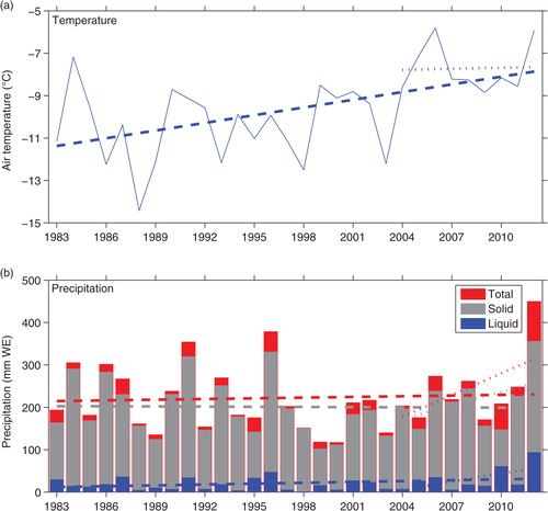
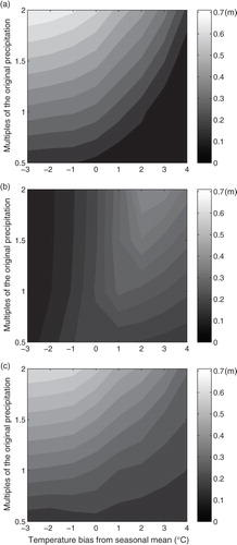
Fig. 9  The maximum slush formation due to (a) flooding and (b) melting, and (c) corresponding maximum ice formed at the ice surface as a function of varying external forcing of air temperature and precipitation. The model is configured with reference model run (Ref) condition.

Anderson E.A. A point energy and mass balance model of a snow cover. NOAA Technical Report 19. 1976; Silver Spring, MD: US Department of Commerce, National Oceanic and Atmospheric Administration, Office of Hydrology.

 Google Scholar