Figures & data
Fig. 1 (a) The modern Arctic Ocean and its constituent seas. Blue arrows indicate the surface circulation and red arrows show the flow of Atlantic Water. Locations and names are given for sediment cores shown in Fig. 6. (b) Physiography of the Arctic with ice sheet extents and associated sea-level lowering during the Last Glacial Maximum (LGM), 21–18 Kya, and (c) near the start of the Holocene, 10 Kya.
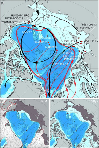
Fig. 2 Major oceanic basins, major rivers and watersheds corresponding to names and basins listed in Supplementary Table S1. The 50-, 100- and 1000-m bathymetric contour levels are shown (from the General Bathymetric Chart of the Oceans, one-minute grid, version 2 (Jakobsson et al. Citation2008). Drainage areas are based on Vorosmarty et al. (Citation2000a, Citationb).
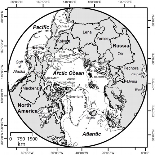
Fig. 3 Trends in precipitation (mm/Ky) between the middle Holocene and 1800 AD (pre-industrial period) for (a) winter (December–January–February), (b) spring (March–April–May), (c) summer (June–July–August) and (d) autumn (September–October–November). Source data from Wagner et al. (Citation2011). A coupled atmosphere–ocean general circulation model, ECHO-G (Legutke & Voss Citation1999), was used to produce the simulation. Trends are calculated using a Mann Kendall Sen slope analytical approach (Yue et al. Citation2002). Trend strength is shown with colours ranging from negative values (brown/yellow tones) to positive values (green/blue tones). Significance is denoted by black circles to represent the 95% confidence interval. Major basins as shown in Fig. 2 are also illustrated.
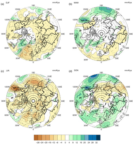
Fig. 4 Modern sediment contribution (Tg y−1) from coastal erosion into the Arctic Ocean divided by marginal sea areas (after Brown et al. Citation2002).
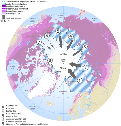
Fig. 5 Holocene sedimentation rates derived from 14C dated sediments and gridded in the Ocean Data View software package (www.odv.awi.de/). The linear sedimentation rates were calculated without using a 0 age assumption for the seafloor.
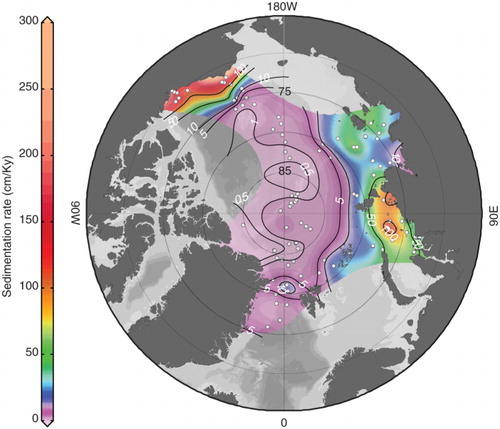
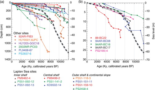
Fig. 6 Global sea level (black and grey dashed line) and published radiocarbon based sedimentation rates in the Arctic. Calibrated radiocarbon data are from Jakobsson et al. (Citation2014) and for the Laptev Sea, Bauch et al. (Citation2001). A subset of available cores was selected where enough radiocarbon dates exist to distinguish between early and late Holocene sedimentation rates. (a) High sedimentation rates are found on continental shelves and slopes across the Arctic, and where dates extend to the base of the Holocene, most seem to capture a period of high sedimentation associated with rapid sea-level rise lasting until 7 Kya. (b) In lower sedimentation rate areas, this trend is not clearly captured by existing records. See Fig. 1 for core locations.