Ice–ocean coupled computations for sea-ice prediction to support ice navigation in Arctic sea routes

Figures & data

Fig. 1  Model bathymetries (m). (a) Whole-Arctic model. To avoid the singularity at the North Pole, the whole-Arctic model grid is rotated to place its North Pole over the equator. Red rectangles denote the high-resolution domains in the Northern Sea Route. (b) High-resolution regional model domain of what in this study we call the Laptev Sea region, consisting of the Laptev Sea and part of the Kara and East Siberian seas, with 50°E–165°E longitudes and 68°N–85.5°N latitudes. (c) High-resolution regional model domain of what we refer to as the Chukchi Sea region, consisting of part of the East Siberian and Chukchi seas, with 154°W–151°E longitudes and 64°N–73.5°N latitudes.

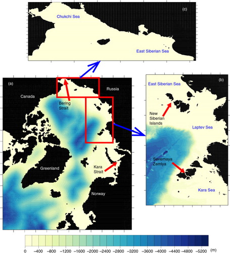
Fig. 2  Ice strength as a function of ice concentration and strain rate parameter Δ with an old formulation (defined in Eqn. 1).

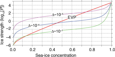
Fig. 3  Ice strength as a function of ice concentration and strain rate parameter Δ with a new formulation (defined in Eqn. 7).

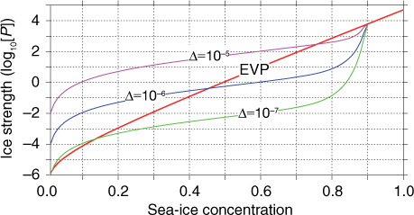
Fig. 4  Sea-ice thickness (m) and the associated ice velocity (m/s) variations from one to four weeks in the two-dimensional test model with (a–d) the old formulation of the coupled ice–ocean model (ice–POM) and (e–h) the new formulation.

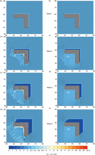
Fig. 5  September mean sea-ice concentration in 2004–2011 from Advanced Microwave Scanning Radiometer–Earth Observing System (AMSR–E) satellite observations, the model and the difference between the model and AMSR–E. The black dots in AMSR–E observations represent missing data.

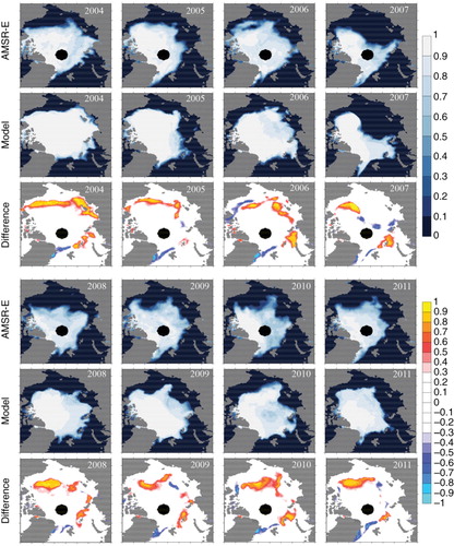
Fig. 6  Daily time series of sea-ice extent in 2001–2011 from the model and satellite observations (Cavalieri et al. 1996).

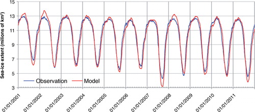
Fig. 7  Interannual and seasonal comparisons between observed Lindsay (2010) mean ice draft and computed model ice draft in four seasons in 2001–2011.

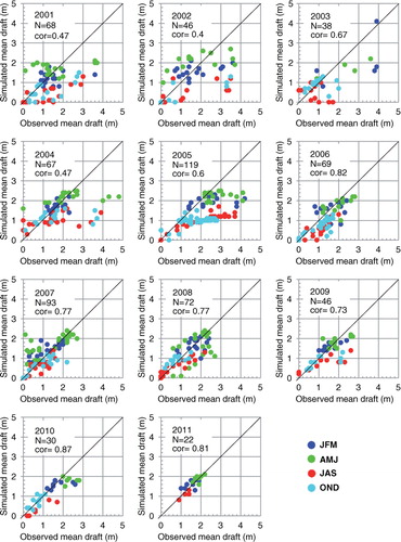
Fig. 8  Comparison of International Arctic Buoy Program drifting buoy motion with modelled ice motion for buoy trajectories N1–N5 in Supplementary Fig. S3. Scatterplots of (a–e) zonal (U) velocity component, and (f–j) the meridional (V) velocity component. Black lines denote the linear fit of the data set and the correlation coefficient is also given with each graph.

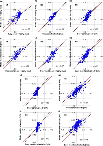
Fig. 9  Sea-ice extent from the whole-Arctic model with coarse grid, the Laptev Sea regional model with fine grid and Advanced Microwave Scanning Radiometer–Earth Observing System (AMSR–E) satellite observations during (a) 20 July 2004 to 17 August 2004 and (b) 20 July 2005 to 17 August 2005. Area covered with ice concentration more than 15% is taken into the comparison.

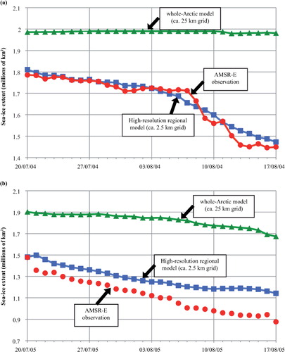
Fig. 10  Sea-ice extent from the whole Arctic model with coarse grid, the Chukchi Sea regional model with fine grid and Advanced Microwave Scanning Radiometer–Earth Observing System (AMSR–E) (Cavalieri et al. 2014) during (a) 20 July 2004 to 17 August 2004 and (b) 20 July 2005 to 17 August 2005. Area covered with ice concentration more than 15% is taken into comparison.

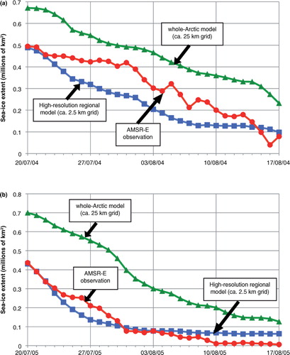
Fig. 11  Sea-ice concentration distribution in the Laptev Sea region from 20 July 2004 to 17 August 2004; upper and middle panels show the model and Advanced Microwave Scanning Radiometer–Earth Observing System (AMSR–E; Cavalieri et al. 2014) satellite-derived concentration and lower figures show difference between model and AMSR–E.

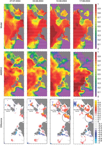
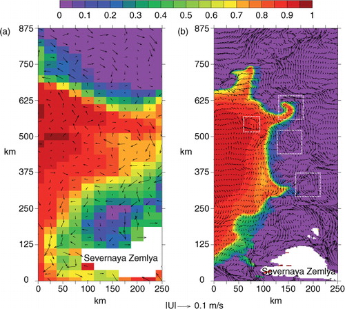
Fig. 12  A snapshot of ice–eddy interaction, sea-ice concentration (colour) and top 100-m average ocean current (vectors) on 1 October 2005 north of the Severnaya Zemlya islands from (a) the whole-Arctic model with a coarser grid (about 25 km) and (b) the regional model with a finer grid (about 2.5 km). Dashed rectangles show some of the mesoscale eddy locations.

Cavalieri D.J., Parkinson C.L., Gloersen P., Zwally H. Sea ice concentrations from Nimbus–7 SMMR and DMSP SSM/I–SSMIS passive microwave data. 1996; Boulder, CO: National Aeronautics and Space Administration Distributed Active Archive Center at the National Snow and Ice Data Center.

 Google Scholar

Lindsay R.W. Unified sea ice thickness climate data record. 2010. Available from the Polar Science Center, Applied Physics Laboratory, University of Washington at psc.apl.washington.edu/sea_ice_cdr.

 Google Scholar

Cavalieri D.J., Markus T., Comiso J.C. AMSR–E/Aqua Daily L3 12.5 km brightness temperature, sea ice concentration, & snow depth polar grids, Version 3. 2014; Boulder, CO: National Aeronautics and Space Administration Distributed Active Archive Center at the National Snow and Ice Data Center.

 Google Scholar