Regional passive seismic monitoring reveals dynamic glacier activity on Spitsbergen, Svalbard

Figures & data

Fig. 1  Location map of the Svalbard archipelago and the main island of Spitsbergen. Glaciers are represented by white areas. Triangles show locations of permanent seismic broadband stations Kings Bay, Ny-Ålesund (KBS), Spitsbergen seismic array (SPITS), Barentsburg (BRBA), Hornsund (HSPB). Stars indicate locations of selected (groups of) glaciers with reported calving activity or surging activity (see text): (1) Smeerenburgbreen, Raudfjordbreen, Waggonwaybreen; (2) Julibreen; (3) Blomstrandbreen; (4) Kronebreen, Kongsbreen; (5) Comfortlessbreen, Aavatsmarkbreen; (6) Osbornebreen, Konowbreen; (8) Tunabreen, Von Postbreen; (9) Nathorstbreen; (10) Vestre/Austre Torellbreen; (11) Storbreen; (13) Hansbreen. The location of the earthquake cluster in Isfjorden is also shown (7), as is the location (12) of the magnitude six earthquakes on 21 February 2008, which experienced ongoing aftershocks for more than five years. Black dots correspond to locations of active coal mines.

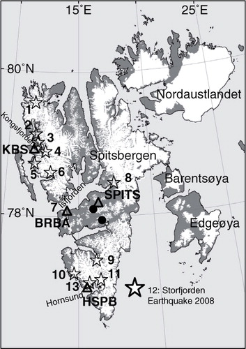
Fig. 2  Uncertainties of seismic event locations obtained with the permanent seismic network on Spitsbergen. In each panel a synthetic source location is assumed representing a real glacier source (circle). P and S travel times as well as backazimuths are modelled at receivers (a–e) at the Kings Bay seismic station (KBS) and the Spitsbergen seismic array (SPITS), (f) SPITS only or (g–i) at the Polish research station at Hornsund (HSPB) and SPITS, using true source location and nodes on a grid of trial locations. Misfit of modelled data at each node is shown as grey scale image. Scale is logarithmic to facilitate evaluation of spatial resolution using shape of error surface close to true source. The location of the error bar is the grid node of lowest misfit. True modelled travel times (TT) and backazimuths (BAZ) were perturbed to assess corresponding bias on best source location (see text). Random perturbation using standard deviations of real data in 100 trials was used to compute error bars. Except in (a), (d) and (e), an additional bias was added to input data to simulate possible bias in real data: (b) 15° SPITS, −20° KBS, 2s Pg KBS, no Sg KBS; (c) 15° SPITS, −30° KBS, 1s Pg KBS, no Sg KBS; (f) 20° SPITS, 1s Sg SPITS, no KBS; (g) 20° SPITS, 1s Pg HSPB, no Sg HSPB; (h) 20° SPITS, 1s Pg HSPB; (i) 20° SPITS, 1 s Pg HSPB, no Sg HSPB.

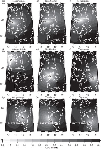
Fig. 3  Example of waveforms (vertical component) of seismic events from different regions in (a–f) north-west and central Spitsbergen and (g–h) southern Spitsbergen. The text colour code is same as in Figs. 4, 5 and 6. Note different scales for y axis. (a), (b), (c), (e) Examples of calving signals of clusters 2–5 in the greater Kongsfjorden region (see Figs. 1, 4). Data are bandpass-filtered from 1.4 to 19 Hz. (d) Example of a non-glacial event in the Isfjorden area (cluster 7). (e) Same calving event recorded at stations at the Kings Bay seismic station (KBS) and the Spitsbergen seismic array (SPITS). (f) Seismic event at Tunabreen (cluster 8, calving). (g) Examples of cluster 9 at Nathorstbreen (glacier surge). (h) Seismic event in the Hornsund area (cluster 10–11, calving). Seismic phase picks used for location and uncertain or multiple arrivals are shown in dark red.

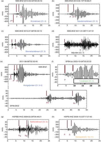
Fig. 4  Seismicity in (a) north-west Spitsbergen and (b) southern Spitsbergen located using manual seismic phase picks on permanent regional network and azimuths measured at the Spitsbergen seismic array (SPITS). The same numbers are used to indicate groups of individual glaciers as in Fig. 1. Corresponding glacier areas are coloured dark grey. Coloured symbols indicate different clusters or types of icequakes. Black symbols are seismic events of tectonic or unknown origin. See text for more details. Years/time period of different text colour represent years when the shown events occurred. In (a) 2009–2013 applies for all clusters. Error bar in the lower left corner is the mean location uncertainty estimate for all events.

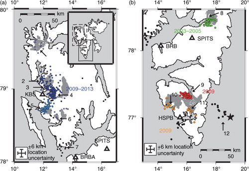
Fig. 5  Average velocity power spectra for the different seismic event clusters shown in Fig. 4 recorded at different stations: (a) the Kings Bay seismic station (KBS), (b) the Spitsbergen seismic array (SPITS) and (c) the Polish research station at Hornsund (HSPB). Blue: cluster 1–5 (Kongsfjorden), black: cluster 7 (Isfjorden, tectonic), green: cluster 8 (Tunabreen), red: cluster 9 (Nathorstbreen), orange: cluster 10–11 (Hornsund). Grey lines show average background noise spectra computed from data windows of same length as events, recorded before each event. In (c) lower noise spectrum corresponds to time period of cluster 9 events only.

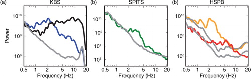
Fig. 6  Temporal distribution of autonomous icequake detections obtained from short-term/long-term average trigger (SLD) or cross-correlation detection method (CCD) applied to regional seismic network stations. The same colour coding is used for seismic clusters as in Fig. 4. Lines and ellipses indicate the range of backazimuth (angle between lines or one axis of ellipse) and distance (other axis of ellipse) of individual source regions as seen in the data from the Spitsbergen seismic array (SPITS). Backazimuth and distance were obtained from frequency-wavenumber analysis of SPITS data for each detection. Distance is assumed to be proportional to time delay between P detection and secondary arrival at SPITS (see text). Distribution of icequake detection with backazimuths and distances falling into this range are shown in histograms presenting event counts with bin width of 10 days. White stars show maximum of days with positive temperatures in July each year. Light grey bars indicate days with data gaps. Seasonal temporal patterns at Kongsfjorden, Tunabreen and Hornsund are the result of glacier calving variability. High seismic activity at Nathorstbreen (2009) and Tunabreen (2003) was related to glacier surges.

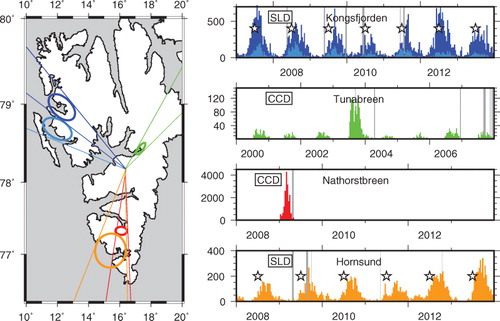
Fig. 7  Comparison between seismic calving events in the greater Kongsfjorden region. (a) Calving events located fully automatically with the Spitsbergen seismic array (SPITS) array in north-western Spitsbergen (SPITS catalogue). Land area is white. (b) Calving events located using manually picked seismic phase arrivals at the Kings Bay seismic station (KBS) and SPITS. This is a subset of locations from Fig. 4 except diamond symbols which were rejected in Fig. 4 because of high RMS errors and no backazimuth measured at KBS. (c) Calving events located using the local network at Kronebreen. Black error bars are location uncertainties. Colour code was chosen from grouping of localizations in (c) and then used for corresponding events in (a) and (b) (different from the colour code in previous figures). Events east (red), south (blue) and north of Kongsfjorden (green) are grouped. Black triangles show locations of seismic receivers. Rectangles in (a) and (b) confine area shown in (c). Except for the event whose source location is shown as a black circle (unknown origin), all events originated at termini of tidewater glaciers.

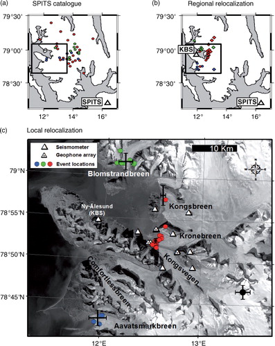
Fig. 8  Percentage of different types of in situ calving observations at Kronebreen matching with seismic event detections at the Kings Bay seismic station (KBS), using the short-term average/long-term-average (STA/LTA) detector. Dashed line: total number of observations was fewer than 10, resulting in less statistical significance. See text for definition of size parameters of in situ observations. Lower calving size limit: for each data point, only calving events having sizes equal or above corresponding size parameter were used for matching. Green triangles show results if only seismic event detections with confirmed locations in the Kongsfjorden region were compared (STA/LTA + frequency-wavenumber analysis, column drops only).

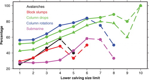
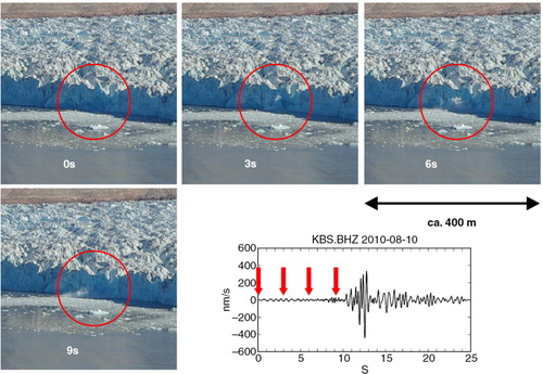
Fig. 9  Example of a calving event at Kronebreen captured on time-lapse camera images on 10 August 2010. A human observer classified this event as a size 2 column drop type. The corresponding seismic signal measured at the Kings Bay seismic station (KBS) in Ny-Ålesund, and filtered between 1.4 and 19 Hz, is shown. Image series and seismic trace start at 09:39:29 UTC. Red vertical arrows indicate timing of images. Travel time between calving front and KBS is 2–6 s, which explains the delay between impact (6 s image) and the signal onset (8–10 s).