The first magnetotelluric image of the lithospheric-scale geological architecture in central Svalbard, Arctic Norway

Figures & data

Fig. 1  (a) Geo-tectonic map of Svalbard redrawn from Dallmann et al. (2002). (b) Schematic regional scale cross-section in a west–east transect across north–central Spitsbergen redrawn from Bergh & Grogan (2003). The portion of the cross-section that is marked by a rectangle corresponds to the magnetotelluric (MT) result shown in Fig. 3b. (c) Station distribution for the measured MT profile, indicated by the rectangle in (a). Geological and other features are abbreviated as follows: Lomfjorden Fault Zone (LFZ); Billefjorden Fault Zone (BFZ); Breibogen Fault (BF); Hornsund Fault Zone (HFZ); the warm springs Trollkildene and Jotunkildene (TJS); Central Tertiary Basin (CTB); Sysselmannbreen (SB); Sassendalen (SD); Longyearbyen CO₂ Lab's well park (LCOP).

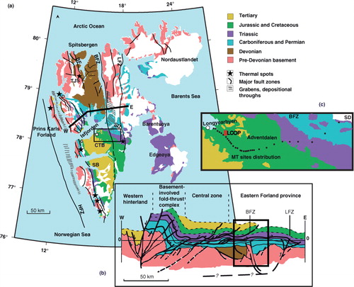
Fig. 2  The dominant regional level geoelectric strike direction with 90° ambiguity and Bahr's three-dimensional/two-dimensional (3D/2D) skew for all the measured 30 stations and the entire measured period range (0.003–1000 s) in log₁₀ (lg) scale. (a) Rose diagram illustrating a regional N30°E geoelectric direction estimated through Bahr's phase-sensitive method. (b) For comparison, a rose diagram displaying a dominant regional strike (N30°E) estimated through the Q-function method, is shown. (c) Bahr's 3D/2D skew parameter as a function of the measured periods. Station-wise data skew parameters (y axis) larger than the empirical threshold of 0.3 may indicate a possible 3D effect, which makes 2D determinant inversion preferable for data interpretation.

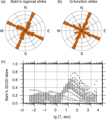
Fig. 3  (a) The final two-dimensional (2D) magnetotelluric (MT) model. The colour scale (lg) is shown in log₁₀. An error floor of 5% is assigned on the inverted data, and the inversion is started from a 100-Ωm half-space model. The data misfit of the final model is shown in Fig. 4. (b) Geological interpretation of the MT model. (c) A schematic geological cross-section derived from a seismic section (parallel to the MT profile) in eastern Isfjorden, redrawn from Blinova et al. (2012). The y axis is given in two-way-travel time (TWT, s), where each second represents two-way-travel time (see Blinova et al. 2012). (d) The offshore seismic transect and the measured MT sites are shown in the same map to illustrate the position of the two profiles in relation to each other. Isfjorden is indicated to facilitate comparison with Fig. 1. The MT result is comparable to interpretations derived from seismic sections as in (c) and to the stratigraphic section marked by the rectangle in Fig. 1b. Geological and other features are abbreviated as follows: Longyearbyen CO₂ Lab's well park (LCOP); permafrost (PF); upper-crust conductive layer (UCL); mid-crust conductor (MCC); resistive layer 1 (RL1); resistive layer 2 (RL2); metamorphic basement (MB).

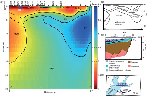
Fig. 4  Pseudo-sections of the misfit between the observed and predicted responses of the determinant data underlying the two-dimensional magnetotelluric model shown in Fig. 3. Sites are sorted in increasing order from left (west) to right (east). Apparent resistivity and period (y axis) are given in log₁₀ (lg) scales, and phase is shown in degrees. The total misfit root mean square of the inversion is 1.06. (a) Observed apparent resistivity. (b) Predicted apparent resistivity. (c) Apparent resistivity misfit. (d) Observed phase. (e) Predicted phase. (f) Phase misfit.

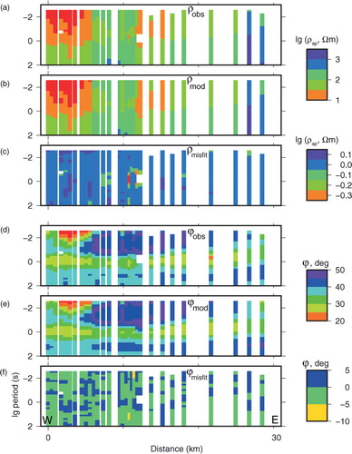
Fig. 5  A two-dimensional model example presented to show the reproducibility of the resistivity geometry seen in the final model (Fig. 3a). We obtained the model by re-running the inversion procedure using 1000-Ωm half space as a starting model with the reduced data space Occam algorithm. This model, which is obtained after eight iterations, has the data misfit root mean square 1.06. The hatched area between the upper-crust conductive layer (UCL) and the mid-crust conductor (MCC) indicates the section of the final model area we tested for sensitivity. The location of resistive layer 2 (RL2) is marked.

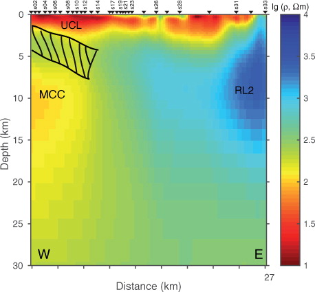
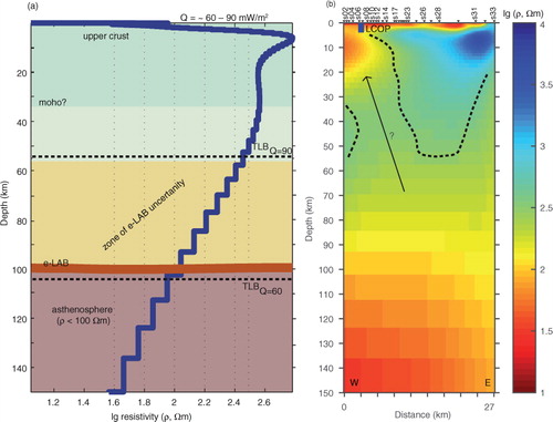
Fig. 6  Resistivity geometry from lithosphere through upper asthenosphere depth. Resistivity values are shown in log₁₀ (lg) scale. (a) One-dimensional regional resistivity stratigraphy obtained from the averaged two-dimensional model shown in (b). Q is the measured surface heat-flow rate, which ranged in value from 60 to 90 mW/m² along the magnetotelluric (MT) profile (Pascal et al. 2011). The depth scale marked as the zone of electrical lithosphere–asthenosphere boundary (e-LAB) uncertainty falls within the calculated upper and lower thermal lithospheric base boundaries (calculated with Eqn. 2) with the specified Q. The Moho depth for Svalbard platform (ca. 30 km) is taken from Faleide et al. (2008)_. (b) The final two-dimensional MT model (Fig. 3) extended down to upper asthenospheric depth. The resistivity geometry marked by the arrow suggests a link between the crustal sedimentary units and the shallow convective mantle. The location of the Longyearbyen CO₂ Lab's well park (LCOP) is marked.

Dallmann W.K., Ohta Y., Elvevold S., Blomeier D. Bedrock map of Svalbard and Jan Mayen. Temakart 33. 2002; Tromsø: Norwegian Polar Institute.

 Google Scholar

Bergh S.G., Grogan P. Tertiary structure of the Sorkapp–Hornsund region, south Spitsbergen, and implications for the offshore southern extension of the fold–thrust belt. Norwegian Journal of Geology. 2003; 83: 43–60.

 Web of Science ®Google Scholar

Blinova M., Faleide J.I., Gabrielsen R.H., Mjelde R. Seafloor expression and shallow structure of a fold-and-thrust system, Isfjorden, west Spitsbergen. Polar Research. 2012; 31 article no. 11209, doi: http://dx.doi.org/10.3402/polar.v31i0.11209.

 Google Scholar

Pascal C., Balling N., Barrere C., Davidsen B., Ebbing J., Elvebakk H., Mesli M., Roberts D., Slagstad T., Willemoes-Wissing B. HeatBar final report 2010. Basement heat generation and heat flow in the western Barents Sea—importance for hydrocarbon systems. Technical report. 2011; Trondheim: Geological Survey of Norway.

 Google Scholar

Faleide J.I., Tsikalas F., Breivik A.J., Mjelde R., Ritzmann O., Engen O., Wilson J., Eldholm O. Structure and evolution of the continental margin off Norway and the Barents Sea. Episodes. 2008; 31: 82.

 Web of Science ®Google Scholar