Figures & data
Fig. 1 Trajectories of buoys A–C, IMB 2010A and historic buoys from 1979 to 2011 drifted from 88° to 80°N, also shown are sea-ice edges from Svalbard to Greenland in March, May and July 2011.
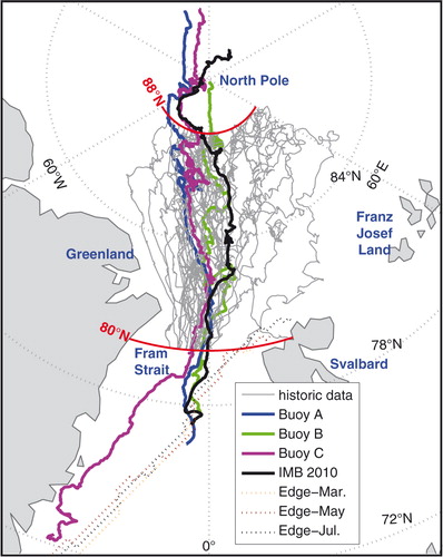
Table 1 Operational history of 2010 buoys.
Fig. 2 Variations in sea-ice velocities measured by buoys A–C and IMB 2010A.
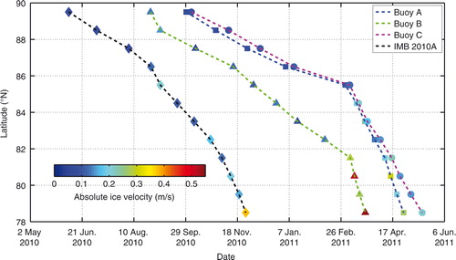
Fig. 3 Monthly correlation coefficients of wind speeds (a) and ice velocities (b) among buoy pairs of A, B and C, and dashed lines represent the 99% significance level.
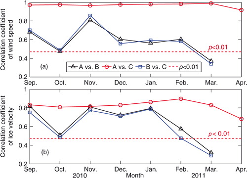
Table 2 Statistical relationships between ice drift and surface wind vectors for the 2010 buoys.
Fig. 4 Monthly direction distributions (%, scaled by numbers in red) of wind heading (black) and ice vector (blue) at buoy A from October 2010 to March 2011, with latitude ranges, MC and DA index in brackets for each panel.
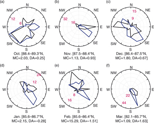
Fig. 5 Amplitudes after Fourier transformation of normalized (a) ice speed scalar and (b) ice velocity vector during times when the amplitudes of 12-h cycle reached the maxima through the buoys’ lives.
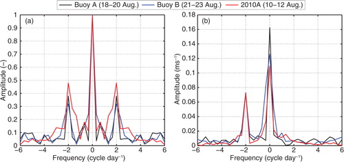
Fig. 6 Amplitude after Fourier transformation corresponding to the 12-h cycle of the normalized velocities of buoys A, B and IMB 2010A for a sliding three-day window and (b, d, e) ice concentrations near the buoys and (a, c, f) the tracks of the buoys when the above-mentioned amplitudes reached the maxima.
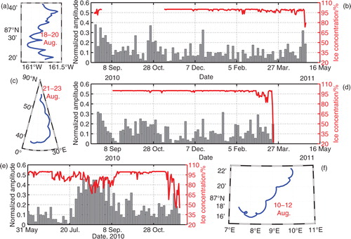
Fig. 7 Trajectories of buoys A, B and C with 30-day positions.
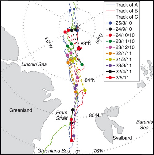
Fig. 8 (a) Distances of buoy pairs among A, B and C, noted that the distance between D and B refers to the right y axis, and others refer to the left y axis; (b) area of the triangle A–B–C; and (c) sea-ice concentration within the triangle A–B–C.
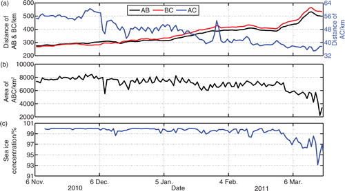
Fig. 9 (a) Seasonal changes in one-latitude average daily ice-drift speed with pluses denoting the time when original data were available, (b) seasonal changes in meridional average ice-drift speed from 85° to 80°N, (c) surface wind speed heading to the north in the section of 60°W to 60°E and (d) meridional changes in averaged ice-drift speed from 80° to 88°N (red for the buoys from 1979 to 2011 and blue for the buoys in 2010).
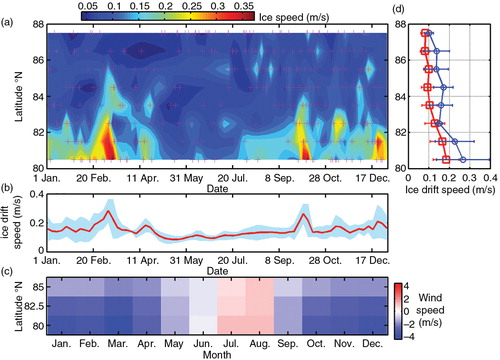
Fig. 10 (a) Monthly DA index (left y axis, black line), travel time from 88° to 80°N of the buoys (right y axis, red line) from 1979 to 2011 and annual Arctic sea-ice area flux through Fram Strait from 1992 to 2007 (right y axis, blue line); (b) linear regression of ice travel time against monthly DA index and (c) linear regressions of year-to-year net increase in summer minimum of Arctic sea-ice extent (left y-axis) and annual Arctic sea-ice area flux through Fram Strait (right y axis) against the travel time of the buoys.
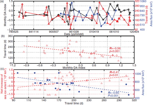
Table 3 Pearson correlation coefficients between pair parameters. Significance levels are P<0.001 (***), P<0.01 (**) and P<0.05 (*); n.s. denotes not significant at the 0.05 significance level.
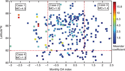
Fig. 11 MC against latitude and monthly DA index for all buoys from 1979 to 2011; the red dashed lines divide the data into four cases: (1) with high negative DA north of 82°N, (2) with neutral DA north of 82°N, (3) with high positive DA north of 82°N and (4) south of 82°N; also shown are the average MCs for various cases; the colour bar for MC was shown at a logarithmic scale.