Estimating sea-ice volume flux out of the Laptev Sea using multiple satellite observations

Figures & data

Fig. 1  Geographic location of the Laptev Sea, modified from Krumpen et al. (2013). The NB and EB used to calculate volume flux are marked as solid black lines. The fast ice edge is indicated as a dashed line. On average, five polynyas are formed between pack ice and fast ice edge, including the New Siberian polynya (NS), the western New Siberian polynya (WNS), the Anabar–Lena polynya (AL), the Taymyr polynya (T) and the Northern Taymyr polynya (NET).

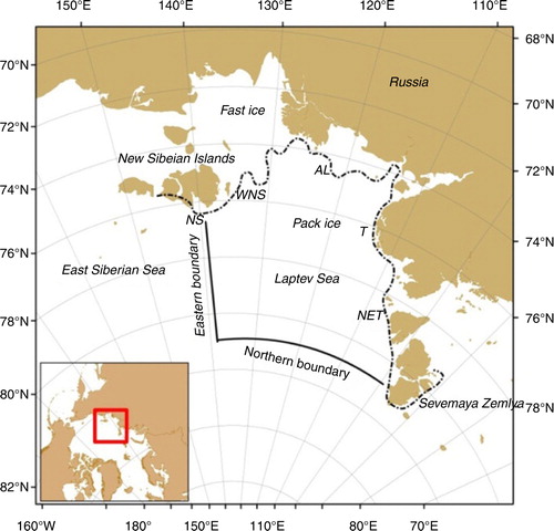
Table 1 Selected values and their uncertainties of input variables used in converting ICESat freeboard to thickness for both periods. See the explanation in the text for how the values were obtained.

Variable	FM/MA	Uncertainty for FM/MA	ON	Uncertainty for ON	References
MY ice density (ρ m )	887 kg/m^3	20 kg/m^3	887 kg/m^3	20 kg/m^3	Eicken et al. 1995
FY ice density (ρ f )	910 kg/m^3	20 kg/m^3	910 kg/m^3	20 kg/m^3	Weeks & Lee 1958; Schwarz & Weeks 1977
Snow density (ρ s )	320 kg/m^3	15 kg/m^3	250 kg/m^3	20 kg/m^3	Kwok & Cunningham 2008
Sea water density (ρ w )	1023.9 kg/m^3	0.5 kg/m^3	1023.9 kg/m^3	0.5 kg/m^3	Laxon et al. 2003
Total ice concentration (c)	AMSR-E 89 GHz	0.05	AMSR-E 89 GHz	0.05	Spreen et al. 2008
MY concentration (c m )	QuikSCAT	0.10	QuikSCAT	0.10	Kwok 2004
Snow depth (s)	MY: W99, FY: AMSR-E	5.9 for FM, 6.2 for MA, 7.0	MY: W99, FY: W99/2	4.2, 7.0	Warren et al. 1999; Brucker & Marku 2013

Fig. 2  Ice-draft comparison between submarine measurements and ICESat retrievals.

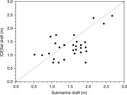
Fig. 3  Spatial distribution maps of estimated uncertainty for sea-ice thickness for the (a) 07FM and (b) 07ON campaign.

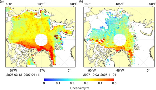
Fig. 4  Representative spatial distribution patterns of ice-drift vectors superimposed on the thickness estimates (blue to red) retrieved from the ICESat measurements. The maps represent the (a) winter and (b) autumn campaigns in 2003. The maps for the 2004–08 period are shown in Supplementary Fig. S2. The red lines represent the location of the two boundaries as indicated in Fig. 1.

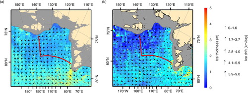
Fig. 5  Ice-drift rate averaged over the Laptev Sea. D _m (in black) and D _z (in red) represent the mean meridional and zonal ice-drift rates, respectively. D _v (in blue) equals to denoting the drift magnitude. The vertical dashed lines are plotted for an easy discrimination drift rates of between autumn (blue) and winter (green) ICESat campaigns. A horizontal black dash line across zero is also given for a clear visual identification of the sign of a drift. A positive (or negative) meridional or zonal value defines a northward (or southward) transport or a westward (or eastward) transport. In other words, a positive (or negative) value indicates that ice is exported out of (or imported into) the Laptev Sea.

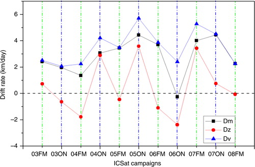
Fig. 6  Time series of sea-ice volume flux estimates through the EB (v _z , orange) and NB (v _m , dark green) boundaries. Blue points denote the total flux (i.e., v _z +v _m ) with error bars showing the uncertainty calculated with Eqn. 8.

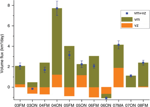
Table 2 Statistics of total volume flux and uncertainty as well as those of the zonal and meridional components across the EB and NB over the investigated period.

Period	EB	Uncertainty for EB	NB	Uncertainty for NB	Total	Uncertainty for the total flux
Winter	−0.06±1.08	0.22±0.05	2.63±0.79	0.60±0.15	2.57±0.91	0.58±0.10
Autumn	0.21±0.93	0.15±0.12	1.74±2.72	0.40±0.10	1.96±3.45	0.41±0.11

Fig. 7  Comparison between ice volume flux estimates through the Laptev Sea and Fram Strait. The Fram Strait outflow was obtained from Spreen et al. (2009).

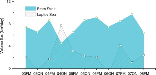
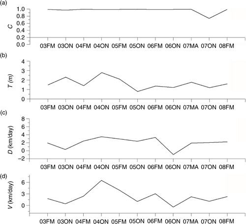
Fig. 8  Time series of volume flux estimates at the NB along with a time series of values of parameters used to obtain the volume flux estimates. This figure represents the variability of sea-ice concentration (c), ice thickness (T), ice-drift rate (D) and ice volume flux (V) over the NB boundary.

Krumpen T., Janout M., Hodges K., Gerdes R., Girard-Ardhuin F., Hölemann J., Willmes S. Variability and trends in Laptev Sea ice outflow between 1992–2011. The Cryosphere. 2013; 7: 1–15.

 Web of Science ®Google Scholar

Eicken H., Lensu M., Leppäranta M., Tucker W.B., Salmela A.J.G.O. Thickness, structure, and properties of level summer multiyear ice in the Eurasian sector of the Arctic Ocean. Journal of Geophysical Research—Oceans. 1995; 100: 22697–22710.

 Web of Science ®Google Scholar

Weeks W.F., Lee O.S. Observations on the physical properties of sea-ice at Hopedale, Labrador. Arctic. 1958; 11: 134–155.

 Google Scholar

Screen J.A., Simmonds I. The central role of diminishing sea ice in recent Arctic temperature amplification. Nature. 2010; 464: 1334–1337.

 PubMed Web of Science ®Google Scholar

Kwok R., Cunningham G.F., Pang S.S. Fram Strait sea ice outflow. Journal of Geophysical Research—Oceans. 2004; 109: C01009,. doi: http://dx.doi.org/10.1029/2003JC001785.

 Google Scholar

Laxon S.W., Giles K.A., Ridout A.L., Wingham D.J., Willatt R., Cullen R., Kwok R., Schweiger A., Zhang J., Haas C., Hendricks S., Krishfield R., Kurtz N., Farrell S., Davidson M. CryoSat-2 estimates of Arctic sea ice thickness and volume. Geophysical Research Letters. 2013; 40: 732–737.

 Web of Science ®Google Scholar

Spreen G., Kwok R., Menemenlis D. Trends in Arctic sea ice drift and role of wind forcing: 1992–2009. Geophysical Research Letters. 2011; 38: L19501, doi: http://dx.doi.org/10.1029/2011GL048970.

 Google Scholar

Kwok R., Cunningham G.F., Wensnahan M., Rigor I., Zwally H.J., Yi D. Thinning and volume loss of the Arctic Ocean sea ice cover: 2003–2008. Journal of Geophysical Research—Oceans. 2009; 114: C07005,. doi: http://dx.doi.org/10.1029/2009JC005312.

 Google Scholar

Zwally H., Schutz B., Abdalati W., Abshire J., Bentley C., Brenner A., Bufton J., Dezio J., Hancock D., Harding D. ICESat's laser measurements of polar ice, atmosphere, ocean, and land. Journal of Geodynamics. 2002; 34: 405–445.

 Web of Science ®Google Scholar

Brucker L., Markus T. Arctic-scale assessment of satellite passive microwave-derived snow depth on sea ice using Operation IceBridge airborne data. Journal of Geophysical Research—Oceans. 2013; 118: 2892–2905.

 Web of Science ®Google Scholar

Spreen G., Kern S., Stammer D., Hansen E. Fram Strait sea ice volume export estimated between 2003 and 2008 from satellite data. Geophysical Research Letters. 2009; 36: L19502,. doi: http://dx.doi.org/10.1029/2009GL039591.

 Google Scholar