Freshwater ostracods (Crustacea) and environmental variability of polygon ponds in the tundra of the Indigirka Lowland, north-east Siberia

Figures & data

Fig. 1  Distribution of polygon landscapes in the Arctic. The study area near the World Wildlife Fund Kytalyk field station in the north-east Siberian Indigirka Lowland is indicated by a red marker. Map kindly provided by Pim de Klerk (Freie Universität Berlin and State Museum of Natural History in Karlsruhe, Germany) and modified after Minke et al. (2007).

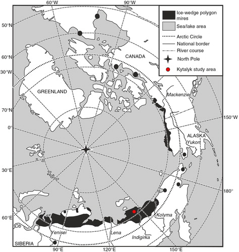
Fig. 2  The study area around the Kytalyk field station (red marker) includes several yedoma ridges, alas depressions located between the western (W) and eastern (E) yedoma ridge, and the Berelekh River floodplain as shown in a panchromatic/multi-spectral imagery satellite image from August 2010 with 0.5 m resolution (GeoEye 4318026). The numbers indicate the pond locations. Courtesy of J. van Huissteden (Vrije Universiteit Amsterdam, Faculty of Earth and Life Sciences, The Netherlands). Map compiled by Mathias Ulrich (Leipzig University, Germany).

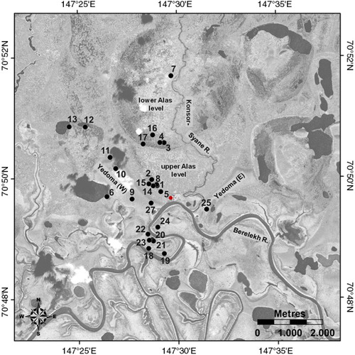
Fig. 3  Monitored site Kyt-01 covered an area of approximately 20×30 m; its central depression accommodated an 11.5×13.5 m wide intrapolygon pond. A boggy moss–sedge zone, polygon walls and frost cracks completely enclosed the pond. The polygon rims rose 0.3–0.4 m above the pond water table. The thaw depth below the pond centre was 40–58 cm while it was 19–24 cm at the polygon rims. (a) Photograph of monitored pond Kyt-01; an arrow indicates the position of the data sensors in the pond centre. View towards the east. Buildings in the background belong to the Kytalyk field station. (b) Schematic top view of the monitoring site with location of the data sensors. Active layer and ground surface elevation were measured along the A–B transect at 1-m resolution. (c) Schematic elevation profile along the A–B transect as measured on 26 August 2011. Zero on the vertical axis indicates the pond water level.

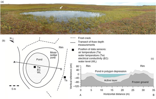
Table 1 Location, type, number and morphometry of the studied polygon water bodies according to major landscape unit and water type.

Landscape unit	n	Length (m)	Width (m)	Water depth (cm)	Thaw depth, pond (cm)	Thaw depth, rim (cm)
Alas	15	8–20	6–21	15–67	18–53	21–65
Yedoma	3	6–10	2–6	22–42	33–45	40
Berelekh River floodplain	9	10–50	5–50	50 to >100	20–45	45–50
Water body type	n	Length (m)	Width (m)	Water depth (cm)	Thaw depth, pond (cm)	Thaw depth, rim (cm)
Intrapolygon pond	12	5–25	7–21	15–70	35–53	21–65
Interpolygon pond	6	9–25	1–6	48–68	18–45	26–55
Thaw lake	3	50–100	10–20	70 to >100	no data	19–48
Other type	6	6–100	2–25	18 to >100	33 to > 100	32–48

Table 2 Species list and counts of individuals per sample of freshwater ostracods from the Indigirka Lowland, north-east Siberia.

Site	Candona mülleri jakutica	Cyclocypris ovum	Cypria exsculpta	F.^a groenlandica	F. harmsworthi	F. krochini	F. pedata	F. protzi	F. sp.	Eucypris sp.	Juvenile Candoninae	Total
Kyt-01-01							2				81	83
Kyt-01-02							8				64	72
Kyt-01-03							19				60	79
Kyt-01-04							22				96	118
Kyt-01-05		1					20				62	83
Kyt-01-06		1					65				39	105
Kyt-01-07							62				60	122
Kyt-01-08	1						44		1		34	80
Kyt-01-09							74				30	104
Kyt-01-10							112				32	144
Total Kyt-01	1	2					428		1		558	990
Kyt-02		1				1	62				107	171
Kyt-03	11					15	21				44	91
Kyt-04		1				7	62				52	122
Kyt-05		1				4	120				30	155
Kyt-06						2	25				37	64
Kyt-07	5						33		6		29	73
Kyt-08	29	1					56		28		1	115
Kyt-09	6	2					12		5		31	56
Kyt-10	68	3		8			372		133		163	747
Kyt-11	3										1	4
Kyt-12						1	54				32	87
Kyt-13	4					1	120				5	130
Kyt-14							382				13	395
Kyt-15	1	1					18		4		2	26
Kyt-16	6						134		6		15	161
Kyt-17					2	1	123				19	145
Kyt-18	16						61		16		1	94
Kyt-19						9	126				87	222
Kyt-20	5	1					122		38		6	172
Kyt-21			1				139		2		0	142
Kyt-22	3	1					22		3		1	30
Kyt-23	7	1					56		12		88	164
Kyt-24		5				5	99				14	123
Kyt-25						28	57				15	100
Kyt-26		1				6	105	27	4	1	36	180
Kyt-27	40								38		12	90
Total Kyt-2-27	204	19	1	8	2	80	2381	27	295	1	841	3859
Total all	205	21	1	8	2	80	2809	27	296	1	1399	4849

^a Fabaeformiscandona.

Fig. 4  Scanning electron microscope images of ostracod valves from the Indigirka Lowland. Cyclocypris ovum: (1) female left valve (LV), (2) female right valve (RV), (3) female RV inner view, (4) female LV inner view; Fabaeformiscandona krochini: (5) female LV, (6) female RV, (7) male LV, (8) male RV; Fabaeformiscandona sp.: (9) female LV, (10) female RV, (11) male LV, (12) male RV; F. pedata: (13) female LV, (14) female RV, (15) male LV, (16) male RV; Cypria exsculpta: (17) carapace; Eucypris sp.: (18) RV; Fabaeformiscandona harmsworthi: (19) female LV, (20) female RV; F. groenlandica: (21) female LV, (22) female RV; Candona muelleri jakutica: (23) female LV, (24) female RV, (25) male LV, (26) male RV; F. protzi: (27) female carapace, left side, (28) female carapace, right side, (29) male LV, (30) male RV.

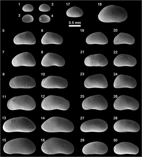
Fig. 5  Ostracod record (number of complete carapaces) from 27 studied water bodies in the Kytalyk area in percent, grouped according to the major landscape units. Note varying scales.

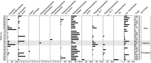
Fig. 6  Non-metric multidimensional scaling biplot of the (a) substrate properties, (b) hydrochemical variables and (c) ostracod species assemblages according to the major landscape units. Environmental parameters are superimposed. Species names are abbreviated as follows: Candona muelleri jakutica (C_m_jak), Cyclocypris ovum (C_ovum), Fabaeformiscandona pedata (F_pedata), F. krochini (F_krochini) and Fabaeformiscandona sp. (F_sp).

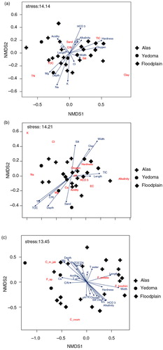
Fig. 7  Population structure of Fabaeformiscandona pedata in the monitored pond Kyt-01 throughout the summer season from 20 July 2011 to 25 August 2011, measured at four-day intervals.

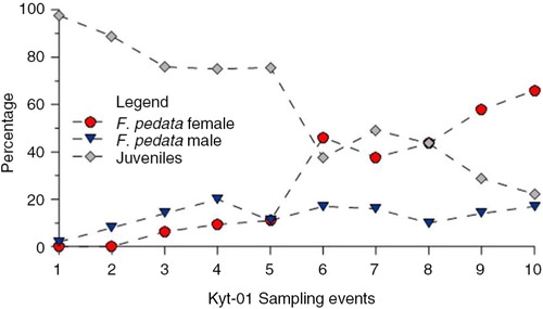
Fig. 8  Monitoring data obtained at the Kyt-01 site from 29 July to 16 August 2011. (a) Air and water temperatures at different depths. (b) Electrical conductivity and water level; rainfall days are marked according to our rainwater sampling for stable isotope analyses and rain gauge measurements (pers. comm. J. van Huissteden, Vrije Universiteit Amsterdam, Faculty of Earth and Life Sciences, The Netherlands). (c) Thaw and water depth in the pond, and thaw depth in the adjacent polygon rim as measured by hand. (d) Selected hydrochemical properties of the monitored pond Kyt-01 obtained during the 10 monitoring events in summer 2011. Note varying scales.

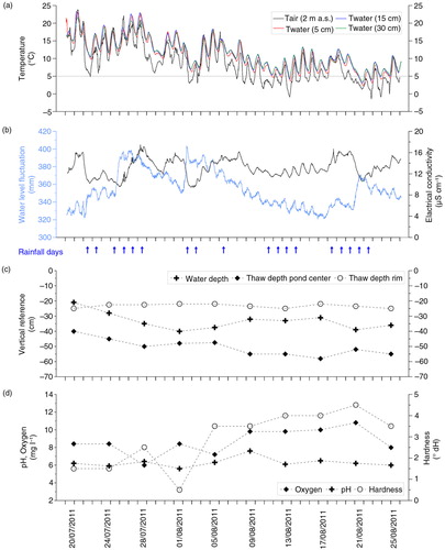
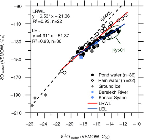
Fig. 9  Stable isotope record of δD and δ¹⁸O from rain and all sampled ponds, ground ice and river water in the Kytalyk study area in summer 2011 relative to the Vienna Standard Mean Ocean Water (VSMOV). Global Meteoric Water Line (GMWL) after Craig (1961). Local evaporation line is abbreviated as LEL and local rain water line as LRWL.

Minke M., Donner N., Karpov N., de Klerk P., Joosten H. Distribution, diversity, development and dynamics of polygon mires: examples from northeast Yakutia (NE Siberia). Peatlands International. 2007; 1: 36–40.

 Google Scholar

Craig H. Isotopic variations in meteoric waters. Science. 1961; 133: 1702–1703.

 PubMed Web of Science ®Google Scholar