Spatial distribution and synoptic conditions of snow accumulation in the Russian Arctic

Figures & data

Fig. 1  Location of meteorological and snow monitoring stations used in this study.

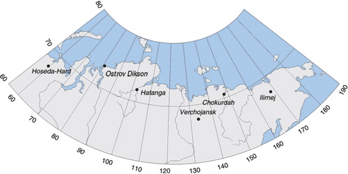
Table 1 Descriptive statistics of snowfall at selected stations across the Russian Arctic (Fig. 1) during the period 1950/51–2012/13.

	Snowfall days		Percent of days with snowfall ≥5 cm		Percentile values of snowfall amount in cm
	≥1 cm	≥5 cm	In total number of days	In number of days with snowfall	90th	95th
Hoseda Hard	2189	505	3.3	23.1	7	5
Ostrov Dickson	1487	278	1.8	18.7	6	4
Hatanga	1233	200	1.3	16.2	5	4
Verhojansk	438	70	0.5	16.0	4	3
Cokurdah	1075	200	1.3	18.6	6	4
Ilirnej	638	169	1.1	26.5	9	5

Fig. 2  (a) Seasonal evolution of daily mean snow depth (cm) at selected stations. (b) Monthly mean snow accumulation (blue) and ablation (red), in cm for the same stations (averages for period 1950/51–2012/13).

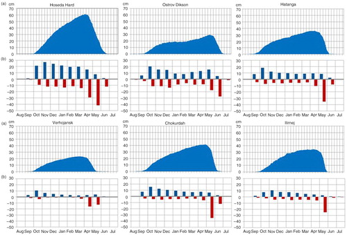
Fig. 3  Mean SLP (hPa) over the Northern Hemisphere during the cold season (October–May) during the period 1950/51–2012/13.

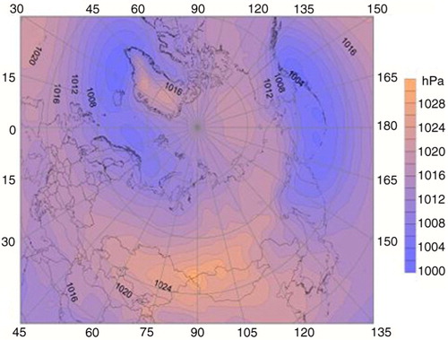
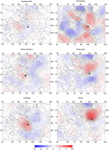
Fig. 4  SLP anomalies for (a) five days prior to and (b) during days of intense snowfall at selected stations.

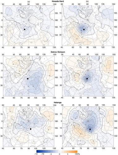
Fig. 5  SLP anomalies for (a) five days prior to and (b) during days of intense snowfall at selected stations.

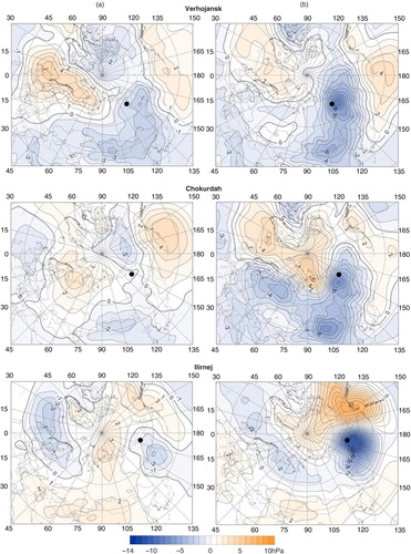
Fig. 6  Spatial distribution of 72-hour backward trajectory end point frequencies for three atmospheric levels: 500 m (red), 2000 m (blue) and 5000 m (green). Based on 72-hour backward air trajectories produced with the HYSPLIT model for the 75 heaviest snowfall days at each station.

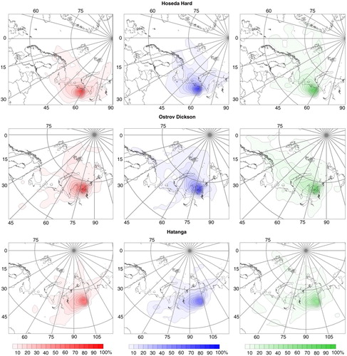
Fig. 7  Spatial distribution of 72-hour backward trajectory end point frequencies for three atmospheric levels: 500 m (red), 2000 m (blue) and 5000 m (green). Based on 72-hour backward air trajectories produced with the HYSPLIT model for the 75 heaviest snowfall days at each station.

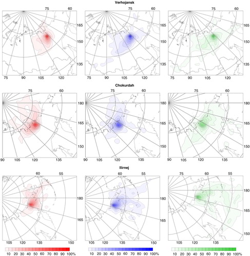
Fig. 8  Anomalies of air temperature at the isobaric level of 850 hPa during days of intense snowfall during winter months (December–February) at selected stations.