Vegetation composition and shrub extent on the Yukon coast, Canada, are strongly linked to ice-wedge polygon degradation

Figures & data

Fig. 1  Location of study area. (a) The studied ice-wedge polygon mires are situated on the Yukon Coastal Plain and Herschel Island within and beyond the reconstructed limit of Quaternary glaciation (white line). Map based on Landsat imagery. (b) Location of study area in North America. (c) Vegetation zones of the wider study region (modified from the Circumpolar Arctic Vegetation Map [CAVM 2013]). (d) Schematic drawing of ice-wedge polygon and measured polygon dimensions.

Table 1 Site characteristics. Medians (boldface) and ranges of the measured sedimentological, hydrochemical and microtopographic parameters are shown for the four investigated polygons. Geographic coordinates are given in decimal degrees in the WGS84 reference coordinate system.

			Substrate
			Particulate portion				Pore water		Microtopography
	Latitude – longitude	Quaternary geology (Rampton 1982)	Texture	TN (%)	TOC (%)	TOC/TN	pH	Electrical conductivity (µS/cm)	Surface height difference within transect (cm)	Active layer depth (cm)	Soil temp. (°C)
Komakuk Polygon intermediate-centred (high-centred)	69.57959 – 140.19853	Lacustrine plain, beyond former glaciation	Peat over sandy clayey silt, coarse sand interspersed	1.8 1.3–2.2	41.3 38.3–44	22.6 18.4–34.6	4.3 3.9–5.7	168 75.1–212.7	29	30.5 26–35	5.1 4–6.7
Roland Polygon high-centred	69.32471 – 139.02092	Rolling moraine	Peat over silty peat	1.1 0.7–1.6	42.6 35.9–44.6	38.7 22.6–62.9	4.0 3.6–4.6	240 90.3–464	20	30.5 22–33	4.2 3.3–6.2
Herschel Polygon low-centred	69.5793 – 138.95740	Push moraine, sea-floor sediment	Sandy silty peat	1.7 0.5–2.1	38.0 26.9–43.6	21.4 14.8–78.7	5.2 4.1–6.2	299 168.6–623	25	32.5 21.5–36	6.5 3–9
Ptarmigan Polygon low-centred	69.49979 – 139.1815	Glacial outwash plain	Sandy silty peat	2.1 0.9–2.4	36.1 30.2–43.3	16.6 14.3–44.7	6.5 4.1–7.3	423 191.1–681	33	25.5 19–31	4.4 1.4–9.8

Fig. 2  The four studied ice-wedge polygons in their settings. Polygon field close-ups on the left are digitized from Geoeye imagery. Ground surface height and permafrost table are shown along transects through each polygon.

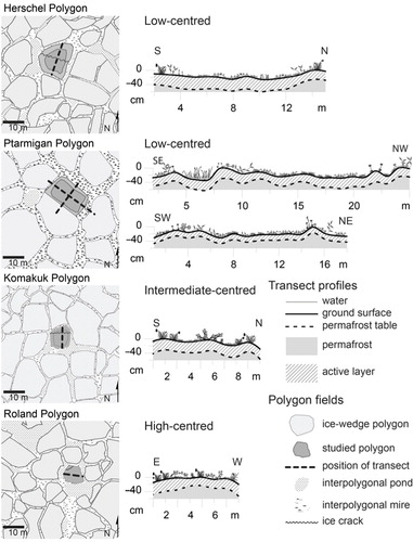
Fig. 3  Surface models of relative height of (a) ground surface, (b) permafrost table, (c) active layer depths and (d) soil temperatures in Ptarmigan Polygon. The blue colour in (b) illustrates an approximation of the position of the water table, which is seasonally and spatially variable because of the underlying permafrost. Plots of 1×1 m named A1 through Q25 are labelled every 2 m.

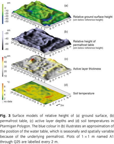
Fig. 4  Vegetation cover and distribution in the studied ice-wedge polygons. (a) The distribution of main plant functional types is linked to relative surface height. Shrub cover is increased on elevated surfaces. Graminoid cover is increased on low-lying surfaces in local depressions. The vegetation cover data are corrected to sum up to 100%. Line graphs below stacked column graphs show the surface height relative to the highest point in each transect. (b) Schematic surface height ranges of shrub species in investigated ice-wedge polygon mires. Ranges are derived from univariate regression tree analysis.

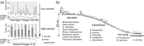
Fig. 5  (a) Vascular plant species composition and abundance differ between the investigated polygons. (b,c) Within low-centred polygons percent cover data of vascular plant species are clearly grouped into taxa related to either low-lying or elevated surfaces. (d) Intermediate-centred and (e) high-centred polygons are more similar. PCA plots show samples, species and environmental parameters. Species scores are indicated by a cross followed by the species name. The points indicate sample scores and the arrows indicate the correlation of environmental parameters with ordination results (only parameters with P<0.05 are shown).

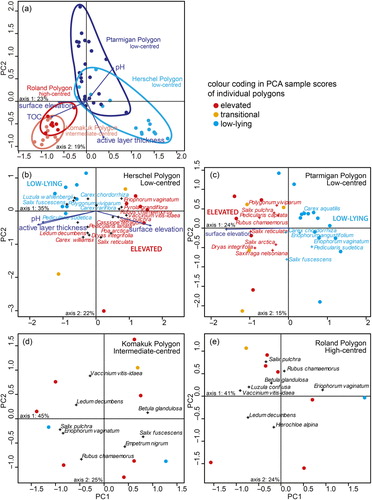
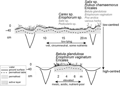
Fig. 6  Schematic diagram showing three main microhabitats of ice-wedge polygon mires (low-centred low-lying, low-centred elevated, high-centred elevated). Dominant vascular plant taxa are indicated for each microhabitat. Permafrost table and ground surface heights are taken from graphically interpolated actual measurements (Supplementary Table S4) every metre. Position, size and depth of ice wedges and ground surface height in the troughs of Roland Polygon are schematic illustrations.

Naito A.T., Cairns D.M. Relationships between Arctic shrub dynamics and topographically derived hydrologic characteristics. Environmental Research Letters. 2011; 6 article no. 045506, doi: http://dx.doi.org/10.1088/1748-9326/6/4/045506 .

 Google Scholar