Air warming trends linked to permafrost warming in the sub-Arctic catchment of Tarfala, Sweden

Figures & data

Fig. 1 Overview map of the Tarfala valley, indicating the location of the Tarfala Research Station (red star), the position of gauges along the Tarfala stream (blue squares) and the three PACE boreholes (pentagons). The topographical catchment boundary is marked by the red line. Elevation difference between isolines is 50 m.

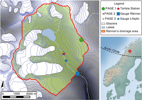
Table 1 Depth (m) of the different thermistors along the PACE-1 borehole. The values are relative to the site's ground surface.

Thermistor depth
0.2	0.4	0.8	1.2	1.6	2	2.5	3	3.5	4	5	7	9	10	11
13	15	20	25	30	40	50	60	70	80	85	90	95	97.5

Fig. 2 Daily observations of ground temperatures (at 0.2 m depth) plotted against corresponding air temperatures at PACE-1 over the period 2000–2011. The data points are sorted in two groups, summer (green) and winter (blue), from which two linear best-fits (red lines) are obtained, and used as estimates of surface ground temperatures.

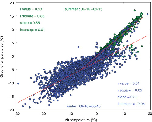
Table 2 Material properties as used in simulations.

	Solid bedrock	Fractured bedrock	Regolith
Hydraulic material properties
Porosity (−)	0.1	0.2	0.4
Rock density (kg/m^3)	3 · 10^3	3 · 10^3	3 · 10^3
Isotropic permeability (m^2)	10^−15	10^−12	10^−10
van Genuchten α (Pa^−1)	10^−4	10^−4	10^−4
van Genuchten λ (−)	0.5	0.5	0.5
Thermal properties
Heat capacity (J·kg^−1·K^−1)	528.0	528.0	528.0
Heat diffusivity (m^2·s^−1)	1.83 · 10^−6	1.83 · 10^−6	1.83 · 10^−6
Thermal conductivity
Rock ( W/(K·m))	2.897	2.897	2.897
Water ( W/(K·m))	0.57	0.57	0.57
Ice ( W/(K·m))	2.2	2.2	2.2
Bulk dry, κ dry (W/(K·m))	1.8011	1.1198	4.3285 · 10^−1
Bulk wet, κ wet,u (W/(K·m))	2.4623	2.0928	1.5118
Bulk frozen, κ wet,f (W/(K·m))	2.8183	2.7418	2.5950

Fig. 3 (a) The attenuation of the annual amplitude of ground temperatures. The amplitude A is defined as the difference between the maximum and minimum temperatures observed in one period (one year) at a given depth z. Annual minima and maxima are emphasized by the horizontal dashed and dashed-dotted lines, respectively. (b) The slope m obtained by fitting a line to the natural logarithm of the annual amplitude ln(A(z)) against depth z. The diffusivity D(m²s⁻¹) is then calculated as D=π·m ²/p where p is the period.

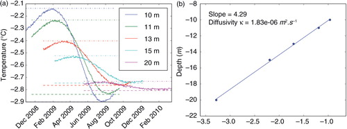
Fig. 4 Temperature time series at 2, 5, 10 and 20 m depth for the time period 2000 to 2011, as measured by PACE-1 borehole thermistors (solid black), and compared with corresponding temperatures obtained from simulation cases T-Air (dashed-dot blue), T-Est (dotted green) and T-Gnd (dashed red).

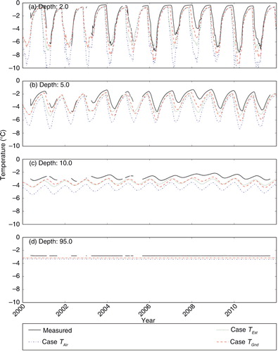
Fig. 5 Measured and simulated temperatures in the shallow ground. Each column of pixels in the colour-charts represents the temperature profile for one day. (a) Observed ground temperatures T _obs (t,z). Three consecutive panes are used to present each scenario: (b), (e) and (h) show the temperature boundary conditions, for cases T-Air (blue), T-Est (green) and T-Gnd (red), with the black thin line representing the daily ground temperature from the 0.2 m thermistor. Panes (c), (f) and (i) are the simulated temperatures T _sim (t,z) and panes (d), (g) and (j) are differences between observations and simulations ΔT(t,z)=T _sim (t,z)−T _obs (t,z). The bottom pane (k) shows the depth integrated absolute as a function of time.

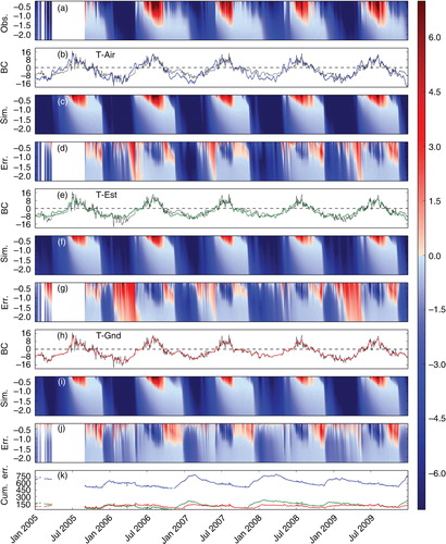
Fig. 6 Ground temperature evolution at 20 m depth. The oscillating curves show the daily ground temperatures. Diamonds show annual averages and the linear curves are trend lines, obtained by linear fit to those averages. The shaded area represents the 95% confidence interval of the estimated trend slope.

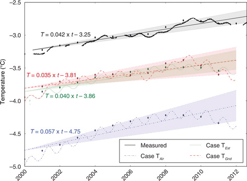
Fig. 7 Slope of linear warming trends at different depth. The shaded area represents the 95% confidence intervals of the slopes obtained by linear best fit to measured data. The case T-Air (blue), T-Est (green) and T-Gnd (red) are represented, as well as a modification of case T-Gnd (cyan), which only differ in that it has a higher heat capacity C_r =600 J·kg⁻¹·K⁻¹.

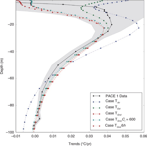
Table 3 Linear regression results for ground temperatures at 20 m depth. The specified intervals are for 95% confidence. The different simulations differ in their boundary conditions: air temperature for T-Air, surface ground temperature for T-Gnd and estimated ground temperature for T-Est.

Simulation	Slope	±	Intercept	±
Measured	0.042	0.008	−3.246	0.055
Simulated
T-Air	0.057	0.019	−4.75	0.12
T-Est	0.040	0.012	−3.86	0.08
T-Gnd	0.035	0.017	−3.8	0.11

Fig. 8 Temperature profiles on 7 June each year, temperatures are from (a) the borehole and (b) the simulation case T-Gnd.

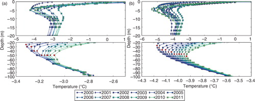
Table 4 Observed and simulated maximum active layer depth (m) for each year.

Year	2000	2001	2002	2003	2004	2005
Data	−1.50	−1.45	−1.47	−1.64	−1.53	−1.54
T-Est	−0.73	−0.64	−0.83	−0.84	−0.73	−0.75
T-Gnd	−0.74	−0.63	−0.89	−0.91	−0.73	−0.74
Year	2006	2007	2008	2009	2010	2011
Data	−1.60	−1.56	−1.50	−1.56	−1.50	−1.58
T-Est	−0.84	−0.74	−0.71	−0.74	−0.72	−0.74
T-Gnd	−0.93	−0.74	−0.64	−0.74	−0.64	−0.84