Figures & data
Fig. 1. Evolution of the temporal weight W t for two consecutive observations.
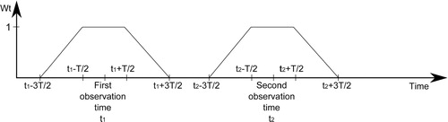
Fig. 2. Evolution of the mean absolute difference between the zonal wind fields of two consecutive iterations, for all the vertical levels influenced by the nudging and all the horizontal grid points, for 10 BFN iterations.
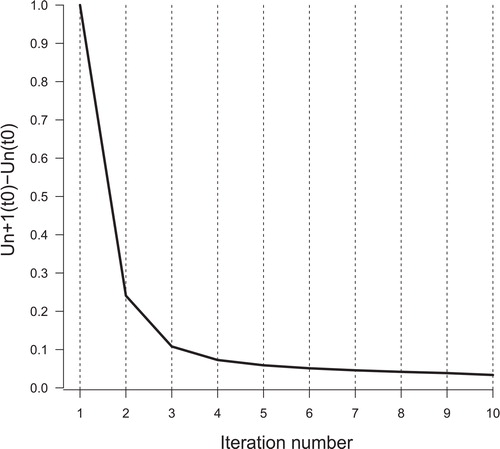
Fig. 3. RMSE between BFN iterations (five iterations) and the true wind profile over the assimilation window (constant wind observation). Each thick solid line represents a direct nudging integration and each thin solid line represents a retrograde nudging integration.
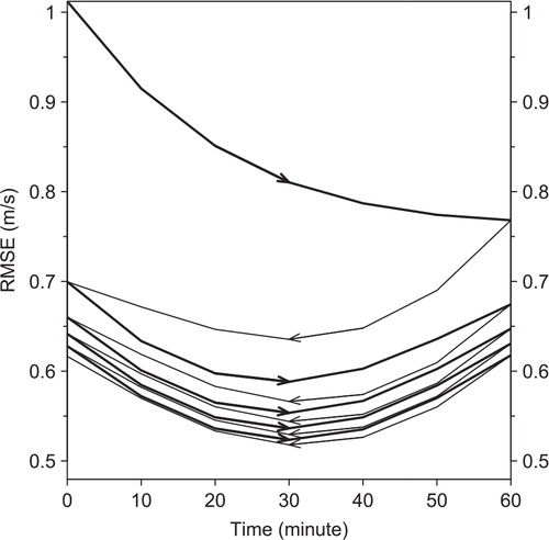
Fig. 4. Observed minus modelled zonal wind at observation location during the BFN iterations (at an altitude of 2000 m). Black bars correspond to values at both ends of the assimilation window, and grey bars correspond to values at the middle of the assimilation window. Vertical lines allow to distinguish between forward and backward model integrations.
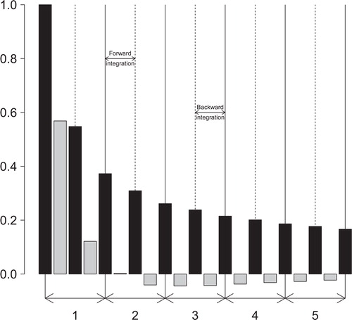
Fig. 5. Evolution of the budget terms (absolute values) from the zonal wind dynamical equations at two model levels (top row = 150 m and bottom row = 2000 m) for three values of the nudging time constant τ (left column = 500 s, middle column = 1000 s and right column = 2500 s). The horizontal axis represents the time over the ten 1-h model integrations (five direct runs and five retrograde runs in alternance). The existence of discontinuities for the turbulence term is the consequence of adiabatic backward integrations ofMeso-NH.
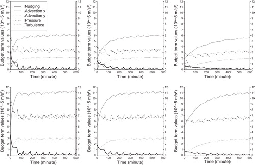
Fig. 6. Wind vector increments at 2000 m during the BFN [first forward integration (a), first backward integration (b), fourth backward integration (c) and fifth forward integration (d)]. Maximum vector represented on each graphic legend corresponds to 1.04 m s−1. The ‘X’ corresponds to the observation location.
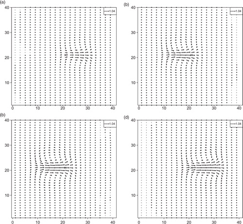
Fig. 7. Same as but for the zonal wind increments.
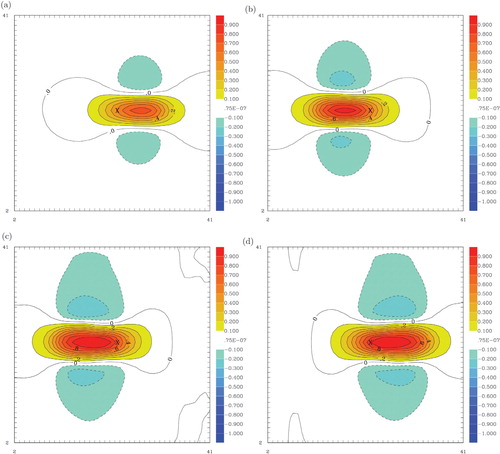
Fig. 8. Influence of the vertical length scale R z on zonal wind profiles at observation location during the first iterations of the BFN. The dashed line indicates the observed profile, the solid line indicates the model profile from a nudging with R z=10 m, the dash-dotted profile indicates the model profile resulting from a nudging with R z=100 m. Top left: profiles at initial time, top right: profiles after one forward integration, bottom left: profiles after one backward integration, bottom right: profiles after the second forward integration.
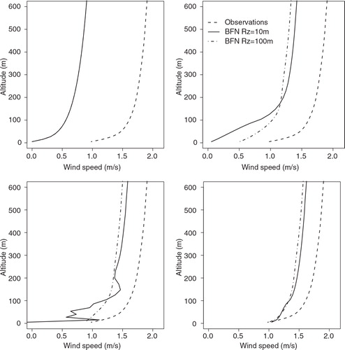
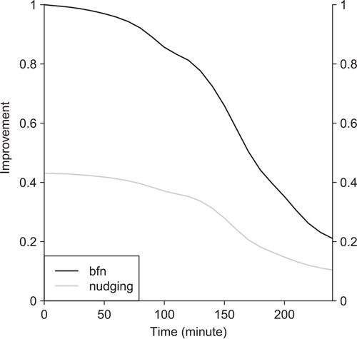
Fig. 9. Improvement factor (departure in RMS from the initial state) during a 4-h forecast after a direct nudging and a BFN (experiment with constant zonal wind).
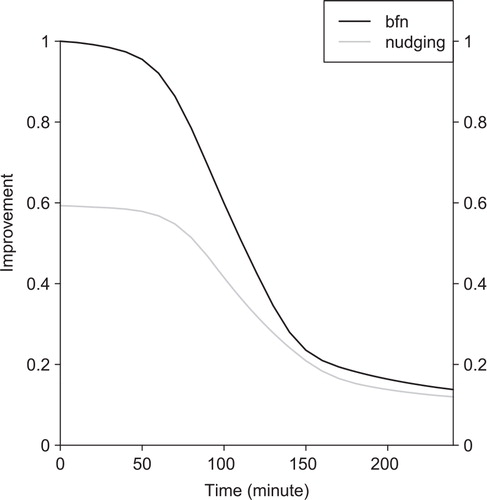
Fig. 10. Wind vector at 2000 m during the BFN iterations with an observation having a 90° rotation in 1 h (from westerly to southerly direction). (a) At initial time, (b) after one forward integration, (c) after two backward integrations and (d) after three forward integrations. Maximum vector represented on each graphic legend corresponds to 1.04 m s−1. The ‘X’ corresponds to the observation location.
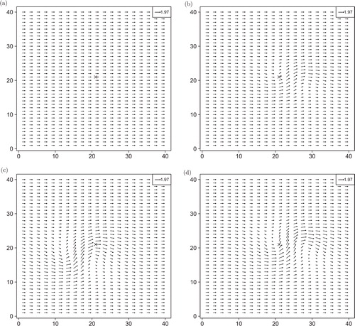
Fig. 11. Improvement factor (departure in RMS from the initial state) during a 4-h forecast after direct nudging and BFN (experiment with wind rotation).