Balanced thermal structure of an intensifying tropical cyclone

Figures & data

Fig. 1.  Plan view of Nuri 1 averaged over the elevation range 5–7 km. The left panel shows the vertical mass flux and the system-relative winds. The right panel shows the Ertel potential vorticity, with black contours indicating zero values. The white dot shows the assumed disturbance centre in the 5–7 km elevation range while the white star shows the storm-relative circulation centre in the 0–2 km range. The red (overall), green (north convective), magenta (south convective) and black (stratiform) boxes define averaging regions to be discussed later.

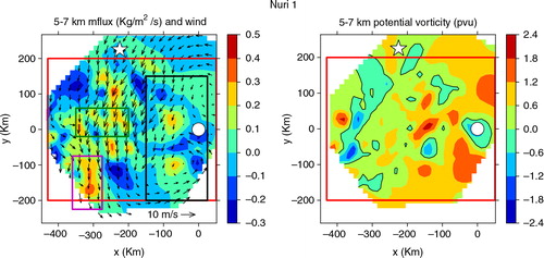
Fig. 2.  Plots of axisymmetry parameter as a function of radius and height for Nuri 1 (left panel) and Nuri 2 (right panel). The radius is defined relative to the 5–7 km centre. Darker shades indicate a closer approach to axisymmetry.

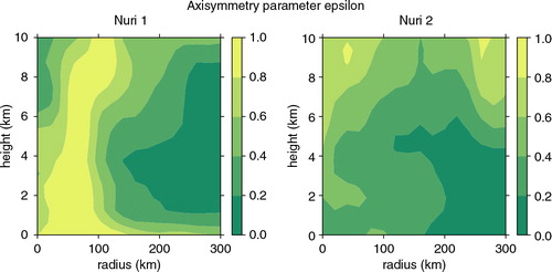
Fig. 3.  Storm-relative zonal (U) and meridional (V) winds as a function of height at the centre of the 5–7 km circulation for Nuri 1 (left panel) and Nuri 2 (right panel).

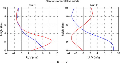
Fig. 4.  Plan view of Nuri 2 averaged over the elevation range 5–7 km. The left panel shows the vertical mass flux and the system-relative winds. The right panel shows the Ertel potential vorticity, with black contours indicating zero values. The white dot shows the assumed disturbance center in the 5–7 km elevation range while the white star shows the storm-relative circulation center in the 0–2 km range. The red (overall), green (central), and magenta (north) boxes define averaging regions to be discussed later.

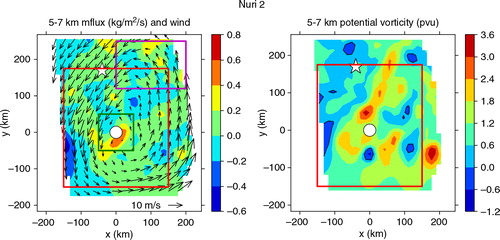
Table 1. Parameters controlling the perturbation potential vorticity and surface potential temperature distributions

Case	i	q i	r i	h i	w i	q Si
Nuri 1	1	1.2 pvu	175 km	5.0 km	4.0 km	−3.5 K
	2	0.1	400	2.0	1.5	0
	3	–1.5	50	6.0	4.5	0
Nuri 2	1	1.3	250	6.0	3.0	–3.0
	2	0.3	400	1.5	2.0	0

Fig. 5.  Comparison of azimuthally averaged potential vorticity (upper panels) and azimuthal wind (lower panels) for observations (left panels) and idealised balance model (right panels). The white region in the upper left panel indicates values of potential vorticity less than −0.4 pvu.

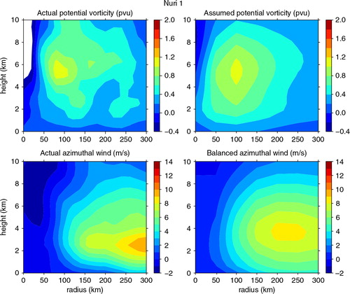
Fig. 6.  Horizontally averaged potential vorticity (upper panel) and virtual potential temperature perturbation (lower panel) for Nuri 1. The thick dashed red line in the upper panel represents the ambient potential vorticity, while the thinner dashed red lines represent areally averaged observations in both panels. The solid blue lines show the averages over a corresponding region in the balanced model result.

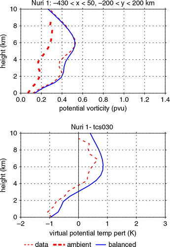
Fig. 7.  East–west section of Nuri 1 meridionally averaged over −200 km ≤ y ≤200 km. The upper panel shows the balance model prediction for the virtual temperature anomaly as a function of x and z. The middle panel shows the observed virtual temperature anomaly (actual Nuri 1 virtual temperature minus the mean virtual temperature for TCS030) while the bottom panel shows the vertical mass flux. The black vertical bars delimit the convective and stratiform regions. Zero contours are represented by thin black lines.

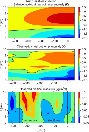
Fig. 8.  North-south section of Nuri 1 zonally averaged over −430 km ≤ x ≤50 km showing the vertical mass flux. The black vertical bars delimit the convective and stratiform regions. Zero contours are represented by thin black lines.

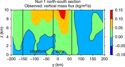
Fig. 9.  Profiles of balanced virtual potential temperature perturbation (thick lines) and observed values (thin dashed lines) (left panel), observed relative humidity (middle panel), and observed vertical mass flux (right panel) for averages over the north convective region (green), south convective region (magenta), and the stratiform region (black), as defined in the left panel of Fig. 1.

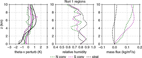
Fig. 10.  Comparison of azimuthally averaged potential vorticity (upper panels) and azimuthal wind (lower panels) for observations (left panels) and idealized balance model (right panels).

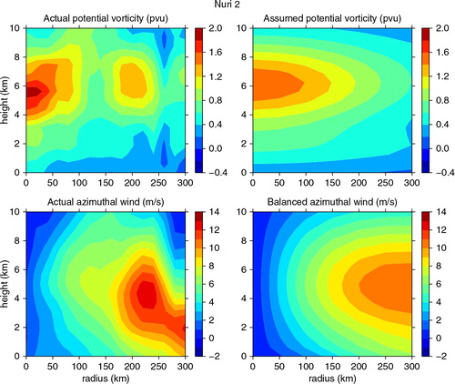
Fig. 11.  Horizontally averaged potential vorticity (upper panel) and virtual potential temperature perturbation (lower panel) for Nuri 2. The thick dashed red line in the upper panel represents the ambient potential vorticity, while the thinner dashed red lines represent areally averaged observations in both panels. The solid blue lines show the averages over a corresponding region in the balanced model result.

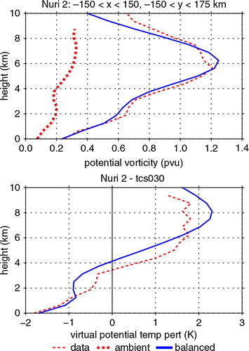
Fig. 12.  East-west section of Nuri 2 meridionally averaged over −150 km ≤ y ≤150 km. The upper panel shows the balance model prediction for the virtual temperature anomaly as a function of x and z. The middle panel shows the observed virtual temperature anomaly (actual Nuri 1 virtual temperature minus the mean virtual temperature for TCS030) while the bottom panel shows the vertical mass flux. The black vertical bars delimit the convective region. Zero contours are represented by thin black lines.

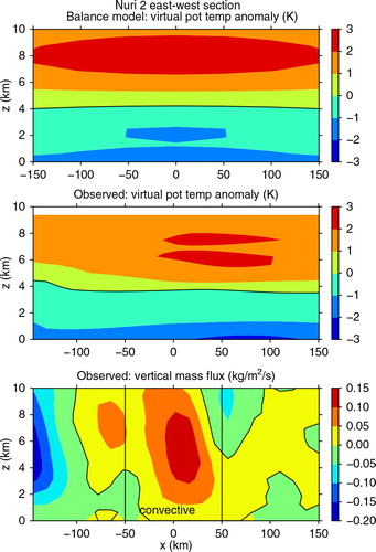
Fig. 13.  North-south section of Nuri 2 zonally averaged over −150 km ≤ x ≤150 km showing the vertical mass flux. The black vertical bars delimit the convective and stratiform regions. Zero contours are represented by thin black lines.

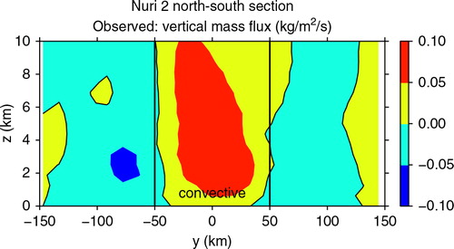
Fig. 14.  Profiles of balanced virtual potential temperature perturbation (thick lines) and observed values (thin dashed lines) (left panel), observed relative humidity (middle panel), and observed vertical mass flux (right panel) for averages over the central (green) and north (magenta) regions of Nuri 2, as defined in the left panel of Fig. 4.

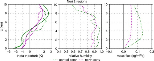
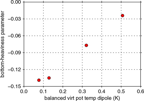
Fig. 15.  Bottom-heaviness parameter B vs. the strength of the balanced virtual potential temperature dipole D for the profiles presented in Figs. 9 and 14.